Index
- Lecture 01
- Lecture 02 Circuit Model of Transmission Line
- Lecture 03 Solution of Wave Equation
- Lecture 04 Reflection Coefficient and Transmission Coefficient
- Lecture 05 Circuit Parameters of a T-line
Lecture 01
Lecture 02
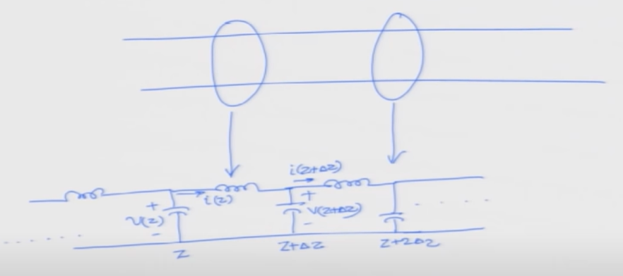
Circuit Model of Transmission Line
- The model only include inductors on the one side.
- However the calculatoin result will be the same
 transmission line model
Using KVL and KCL for the model
\[\begin{align} v(z) + L \Delta z \frac{\partial i(z,t)}{\partial t} + v(z+\Delta z) &= 0\\ i(z) - i(z+\Delta z) - C \Delta z \frac{\partial v(z+\Delta z)}{\partial t} &= 0 \end{align}\]that is
\[\begin{align} \frac{\partial v(z,t)}{\partial z} &= -L \frac{\partial i(z,t)}{\partial t}\\ \frac{\partial i(z,t)}{\partial z} &= -C \frac{\partial v(z,t)}{\partial t} \end{align}\]that is
\[\begin{align} \frac{\partial^2 v}{\partial z^2} &= LC \frac{\partial^2 v}{\partial t^2}\\ \frac{\partial^2 i}{\partial z^2} &= LC \frac{\partial^2 i}{\partial t^2} \end{align}\]Lecture 03
Solution of Wave Equation
For the wave equation like the form
\[\begin{align} \frac{\partial^2 v}{\partial z^2} &= LC \frac{\partial^2 v}{\partial t^2} \end{align}\]the solution is \(v(t,z) = f(t - \sqrt{LC} z)\) or \(v(t,z) = f(t + \sqrt{LC} z)\) with reasonable \(f(.)\)
if
\[v(t,z) = f(t-\sqrt{LC}z)\]then the wave is travelling to the positive direction of \(z\), with phase velocity
\[\mu_{p} = \dfrac{\Delta z}{\Delta t} = \dfrac{1}{\sqrt{LC}}\]e.g.,
\[v(t,z) = \cos(\omega t - \beta z)\]where
\[\dfrac{\omega}{\beta} = \dfrac{1}{\sqrt{LC}}\]Phasor Representation
If we assume all the signal have the same angular frequency \(\omega\), we can represent the signal by phasor. e.g., if the wave is transmited to the positive side of \(z\) axis,
\[\begin{align} V(z) &= V_0^{+} e^{-j\beta z}\\ I(z) &= I_0^{+} e^{-j\beta z} \end{align}\]is the phasor representation of $v(z,t) = V_0^{+}\cos(\omega t - \beta z)$, and \(i(z,t) = I_0^{+}\cos(\omega t - \beta z)\)
using equation
\[\begin{align} \frac{\partial v(z,t)}{\partial z} &= -L \frac{\partial i(z,t)}{\partial t}\\ \end{align}\]we can get
\[\begin{align} I_0^+ &= \dfrac{V_0^+}{Z_0}\\ Z_0 &= \sqrt{\frac{L}{C}} \end{align}\]the \(\sqrt{L/C}\) is called characteristic impedance of the transmission line.
Lecture 04
Reflection Coefficient
assume the wave is the superposition of two directions
\[\begin{align} \widetilde{V}(z) &= V_0^+ e^{-j\beta z} + V_0^- e^{j \beta z} \end{align}\]then using equation
\[\begin{align} \frac{\partial v(z,t)}{\partial z} &= -L \frac{\partial i(z,t)}{\partial t}\\ \end{align}\]we can get
\[\begin{align} \widetilde{I}(z) &= I_0^{+} e^{-j\beta z} + I_0^{-} e^{j\beta z}\\ &= \dfrac{V_{0}^+}{Z_0} e^{-j\beta z} - \dfrac{V_0^-}{Z_0} e^{j\beta z} \end{align}\]now assume we put a load \(Z_L\) at \(z=0\) (the wave is coming from negative infinity size)
\[\begin{align} \widetilde{V}(z=0) &= V_0^{+} + V_0^- = V_L\\ \widetilde{I}(z=0) &= \dfrac{V_0^+}{Z_0} - \dfrac{V_0^-}{Z_0} = I_L\\ Z_L &= \dfrac{V_L}{I_L} \end{align}\]from the equations we can get load reflection coefficient \(\Gamma_L\)
\[\Gamma_L = \dfrac{V_0^-}{V_0^+} = \dfrac{Z_L-Z_0}{Z_L+Z_0}\]- if \(Z_L = \infty\) (the T-line is terminated by open circuit)
and
\[\begin{align} \widetilde{V}(z) &= V_0^+ (e^{-j\beta z} + e^{j\beta z}) = 2 V_0^+ \cos\beta z\\ v(z,t) &= 2 V_0^+ \cos\beta z\cdot \cos\omega t \end{align}\]the above is a standing wave.
- if \(Z_L = 0\) (the T-line is terminated by short circuit)
and
\[\begin{align} \widetilde{V}(z) &= V_0^+(e^{-j\beta z} - e^{j\beta z}) = -2jV_0^+ \sin \beta z \end{align}\]- if \(Z_L = Z_0\)
Transmission Coefficient
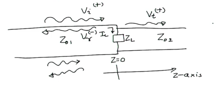 transmission coefficient model
In the model we didn’t consider the reflected wave after \(Z_L\), since we assume the next load is at infinty, thus it will take very long time to reflect back. We already made calculation for \(V_i^+\) and \(V_r^-\) if there is a \(Z_L\). Now we want to determine \(V_t^+\).
\[\begin{align} V_i^+(z=0) + V_r^-(z=0) &= V_L = V_t^+(z=0)\\ \dfrac{V_i^+(z=0)}{Z_{01}} - \dfrac{V_r^-(z=0)}{Z_{01}} &= I_L + \dfrac{V_t^+(z=0)}{Z_{02}} \end{align}\]you can get reflection coefficient
\[\begin{align} \dfrac{V_r^+(z=0)}{V_i^+(z=0)} &= \Gamma_L = \dfrac{Z_{L\Vert} - Z_{01}}{Z_{L\Vert} + Z_{01}} \end{align}\]where
\[Z_{L\Vert} = \dfrac{Z_L Z_{02}}{Z_L + Z_{02}} = Z_L \Vert Z_{02}\]and transmission coefficient
\[\tau = \dfrac{V_t^+(z=0)}{V_i^+(z=0)} = \dfrac{2Z_{L\Vert}}{Z_{L\Vert} + Z_{01}}\]Lecture 05
A Paradox Example
Assume a ideal voltage source (at \(z=-l\)) with voltage \(V_s \cos \omega t\) to drive a lossless T-line. The other end (at \(z=0\)) is terminated by a scope (with infity impedance).
For the open circuit termination, reflection coefficient is 1, and
\[\begin{align} \widetilde{V}_{line}(z) &= 2 V_0^+ \cos \beta z \end{align}\]thus at \(z = 0\)
\[v(t) = 2 V_0^+ \cos\omega t\]at \(z = -l\)
\[v(t) = 2 V_0^+ \cos \beta l \cdot \cos \omega t = V_s \cos \omega t\]thus
\[\begin{align} 2V_0^+ &= V_s / \cos\beta l \end{align}\]then by choosing some \(l\), e.g., \(\beta l=\pi/2\) ,you can get infinity amplified voltage at the scope.
Real Voltage Source
Ideal voltage source doesn’t exist (otherwise it can provide infinity power to drive a short circuit load).
Now we assume the voltage source \(\widetilde{V}_{s}\) is followed by impedance \(Z_s\). And the load is modeled by \(Z_L\).
\[\widetilde{V}_s = \widetilde{I}_{line}(-l) \cdot Z_s + \widetilde{V}_{line}(-l)\]if we assume \(Z_s = \infty\) (open circuit), we know \(\Gamma_L = 1\), and
\[\begin{align} V_0^+ &= V_0^-\\ \widetilde{V}_{line}(z) &= 2 V_0^+ \cos \beta z\\ \widetilde{I}_{line}(z) &= \dfrac{V_0^+}{Z_0} e^{-j\beta z} - \dfrac{V_0^-}{Z_0} e^{j\beta z}\\ &= \dfrac{V_0^+}{Z_0} e^{-j\beta z} - \dfrac{V_0^+}{Z_0} e^{j\beta z} \end{align}\]if we assume \(\beta l = \pi/2\)
\[\widetilde{V}_s = 2 j \dfrac{V_0^+}{Z_0} \cdot Z_s\]and
\[V_0^+ = -j\dfrac{Z_0}{2Z_s} \widetilde{V}_s\]Line Impedance and Input Impedance
we know
\[\begin{align} \widetilde{V}_{line}(z) &= V_0^+ e^{-j\beta z} + V_0^- e^{j\beta z}\\ \widetilde{I}_{line}(z) &= \dfrac{V_0^+}{Z_0} e^{-j \beta z} - \dfrac{V_0^-}{Z_0} e^{j \beta z} \end{align}\]define line impedance (note the difference between line impedance and characteristic impedance)
\[\begin{align} Z_{line}(z) &= \dfrac{\widetilde{V}_{line}(z)}{\widetilde{I}_{line}(z)}\\ &= \dfrac{V_0^+ e^{-j\beta z} + V_0^- e^{j\beta z}}{\dfrac{V_0^+}{Z_0} e^{-j \beta z} - \dfrac{V_0^-}{Z_0} e^{j \beta z}} \end{align}\]thus we can find the input impedance
\[Z_{in} = Z_{line}(-l)\]using
\[\begin{align} V_0^- &= \Gamma_L V_0^+\\ \Gamma_L &= \dfrac{Z_L - Z_0}{Z_L + Z_0} \end{align}\]we have
\[\begin{align} Z_{in} &= Z_0 \Bigg( \dfrac{Z_L \cos \beta l + j Z_0 \sin \beta l}{Z_0 \cos \beta l + j Z_L \sin \beta l} \Bigg)\\ &= Z_0 \Bigg( \dfrac{Z_L + j Z_0 \tan \beta l}{Z_0 + j Z_L \tan \beta l} \Bigg) \end{align}\]we call \(\beta l\) as electrical length.
Example
A voltage source \(V_s = 10 \cos (\omega t + \pi/6)\), or phasor \(10 \cdot e^{j \pi/6}\)