For a \(n\)-th order system
\[H(s) = \frac{a_0 + a_1 s + a_2 s^2 + \dots + a_m s^m}{1 + b_1 s + b_2 s^2 + \dots + b_n s^n}\]A typical circuit will have transfer function with \(\omega_{l}\) and \(\omega_{h}\). And between the two frequencies, the gain is flat \(a_{mid}\)
Bandwidth Estimation Using \(b_1\) Coefficient
- A paper (which paper?) shows that \(1/b_1\) is always smaller than \(\omega_h\).
Example 01
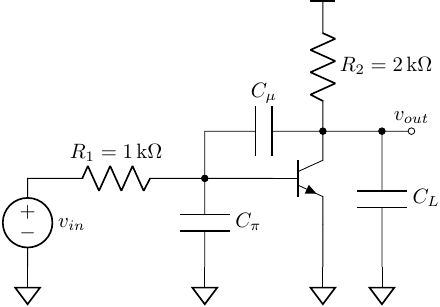 Example 01
Ignore \(r_o\) of the transistor and let
\[\begin{align} C_{\pi} &= 100 fF \quad \quad \quad r_{\pi} = 2.5 k\Omega \\ C_{\mu} &= 20 fF \quad \quad \quad \,\, g_{m} = 40 mS\\ C_{L} &= 200 fF \quad \quad \quad \beta = 100 \end{align}\]the time constants
\[\begin{align} \tau_{\pi}^{0} &= (R_1 \Vert r_{\pi}) C_{\pi} = (1k\Omega \Vert 2.5k\Omega) \cdot 100 fF = 70 ps\\ \tau_{\mu}^{0} &= (R_{left} + R_{right} + G_m R_{left} R_{right}) C_{\mu} = 1200 ps\\ \tau_{L}^{0} &= R_2 C_L = 400 ps \end{align}\]thus
\[\begin{align} b_1 &= \tau_{\pi}^{0} + \tau_{\mu}^{0} + \tau_{L}^{0} = 1670 ps\\ \omega_{h} &= \frac{1}{b_1} = 2 \pi \times 95 MHz \end{align}\]\(\omega_{l}\) is not shown in the model.
$\square$
Bandpass Model
The reactive elements can be divided into two (non-overlap) groups:
- one is responsible for \(\omega_l\)
- another one is responsible for \(\omega_h\)
- so we got two different circuits to calculate \(\omega_{l}\) and \(\omega_{h}\)
For \(\omega_{h}\) we use zero value time constant (ZVT), meaning all the other elements are at zero value.
\[\begin{align} \omega_h \approx 1/b_1 = \frac{1}{\sum_{i=1}^{N} \tau_{i}^{0}} \end{align}\]For \(\omega_{l}\) we use infinite value time constant (IVT), meaning all the other elements are at infinite value.
\[\begin{align} \omega_{l} \approx \frac{b_{n-1}}{b_n} = \sum_{i=1}^{M} \frac{1}{\tau_{i}^{\infty}} \end{align}\]Example 02
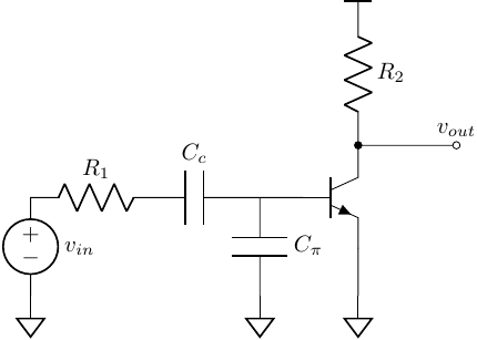 Example 02
$\square$
Taking Zeros Into Account
From Lecture and Paper by Prof. Ali Hajimiri.
\[\omega_h \approx \frac{1}{\sum_{i=1}^{N} \tau_i^{0} (1 - |\frac{H^i}{H^0}|)}\]Not very sure about the proof of this approximation (modified time constant)!
Example 03
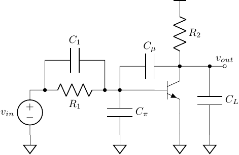 Example 03
Try to make \(C_1\) smaller!
\[\begin{align} C_1 &= 4.3 pF \quad \quad \, \, r_{\pi} = 2.5 k\Omega\\ C_L &= 200 fF \quad \quad g_m = 40 mS\\ C_{\pi} &= 100 fF \quad \quad R_1 = 1 k\Omega\\ C_{\mu} &= 20fF \quad \quad \, \, R_2 = 2 k\Omega \end{align}\]If using bandpass model, and let \(C_1\) being coupling capacitor.
\[\begin{align} b_1 &= R_2 (C_{\mu} + C_{L}) = 440 ps\\ \omega_{h} &= \frac{1}{b_1} = 2\pi \times 362 MHz\\ \tau_{1}^{\infty} &= (R_1 \Vert r_{\pi}) C_1 = 3ns\\ \omega_{l} &= \frac{1}{\tau_{1}^{\infty}} = 2\pi \times 53 MHz \end{align}\]If using modified time constant
\[\begin{align} H^{0} &= -\frac{r_{\pi}}{R_1 + r_{\pi}} \cdot g_m R_2 = -57 \\ H^{\pi} &= 0\\ H^{\mu} &= + \frac{r_m \Vert R_2}{R_1 + r_m \Vert R_2} = 24 m\\ H^{L} &= 0\\ H^{1} &= -g_m R_2 = -80 \end{align}\]with
\[\begin{align} \tau_{\pi}^{0} &= (R_1 \Vert r_{\pi}) C_{\pi} = (1k\Omega \Vert 2.5k\Omega) \cdot 100 fF = 70 ps\\ \tau_{\mu}^{0} &= (R_{left} + R_{right} + G_m R_{left} R_{right}) C_{\mu} = 1200 ps\\ \tau_{L}^{0} &= R_2 C_L = 400 ps\\ \tau_{1}^{0} &= (R_1 \Vert r_{\pi}) C_1 = 3070 ps \end{align}\]modified time conetant
\[\begin{align} \tau_{\pi}' &= 70ps\\ \tau_{\mu}' &= 1200ps\\ \tau_{L}' &= 400ps\\ \tau_{1}' &= -1200ps \end{align}\]then
\[\begin{align} \omega_h = 2\pi \times 339 MHz \end{align}\]$\square$