In this post, the principle of DC analysis, AC analysis and transient analysis are explained. We will focus on the minimum examples, such that the algorithms can be simplified as much as possible. In the later posts, the algorithms for more complicated scenarios will be introduced.
References:
- Paper: Elements of Computer-Aided Circuit Analysis
- Book: Electronic Circuit and System Simulation Methods
DC Analysis
For Linear Circuits
Linear circuits are composed of resistors, capacitors, inductors, independent and dependent sources. In the minimum example in this section, we assume the circuits are only compsed of linear resistors and independent current sources, and they are time-invariant.
Nodal analysis are applied to the linear DC analysis. For a circuit of \(N\) nodes, the number of equations (or the dimension of the voltage vector) will be \(N-1\), since one of the node will be selected as the ground reference. Assume we lable the nodes from \(0\) to \(N-1\), where node \(0\) is the ground reference (\(V_0 = 0\)).
For node \(i (i \ne 0)\), let \(I_i\) be the total current flowing into the node \(i\) from the independent current sources. Let \(V_i\) be the voltage level at node \(i\). The equation for node \(i\) is
\[I_i + \sum_{0 \le k \le N-1, k \ne i} G_{ik} (V_k - V_i) = 0\]That is
\[(\sum_{0 \le k \le N-1, k\ne i} G_{ik}) V_i - \sum_{1 \le k \le N-1, k\ne i} G_{ik} V_k = I_i\]The \(N-1\) equations will be
\[\begin{bmatrix} Y_{11} & Y_{12} & \dots & Y_{1(N-1)}\\ Y_{21} & Y_{22} & \dots & Y_{2(N-1)}\\ \vdots & \vdots & \ddots & \vdots\\ Y_{(N-1)1} & Y_{(N-1)2} & \dots & Y_{(N-1)(N-1)} \end{bmatrix} \begin{bmatrix} V_{1}\\ V_{2}\\ \vdots\\ V_{N-1} \end{bmatrix}= \begin{bmatrix} I_{1}\\ I_{2}\\ \vdots\\ I_{N-1} \end{bmatrix}\]or in short
\[YV=I\]The \(Y\) matrix is called nodal admittance matrix. Let \(G_{ik}\) be the conductance of the resistor connected between node \(i\) and \(k\) (\(i\ne k\)), then the \(Y\) matrix can be calculated as
\[Y_{ij}= \begin{cases} \sum\limits_{0\le k \le N-1, k\ne i} G_{ik}, \quad &\text{ if } i = j\\ -G_{ij}, \quad &\text{ if } i \ne j \end{cases}\]Each \(V_i\) is the voltage level (to be determined) at the node \(i\). \(I_i\) is the total current flowing into the node \(i\) from the independent current sources. The circuit is solved by
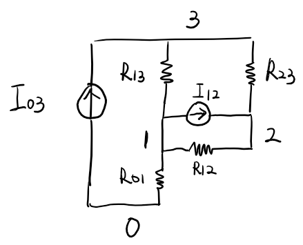
\[V = Y^{-1}I\]Example:
For Nonlinear Circuits
Take the following example. The diode can be viewed as a nonliear voltage controlled resistor.
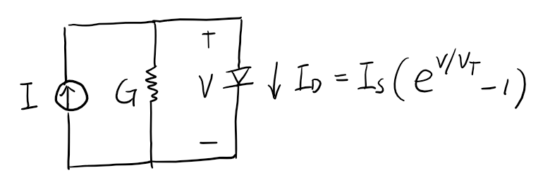
where
\[\begin{align} I_{k} &= I_s(e^{V_k/V_T}-1) - V_k g_k\\ g_k &= \dfrac{\partial I_{D}}{\partial V} \bigg\vert_{V=V_k} = \dfrac{I_s}{V_T}e^{V_k/V_T} \end{align}\]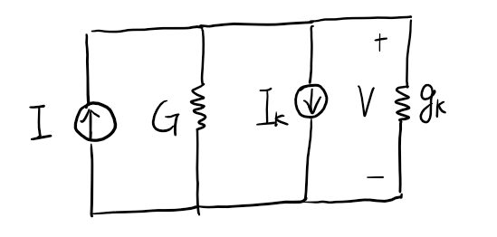
Then by nodal analysis
\[(G+g_k) V = I - I_k\]This is an iterative procedure
\[\begin{align} V_{k+1} &= \dfrac{I-I_k}{G+g_k}\\ &= \dfrac{I-I_s(e^{V_k/V_T}-1) - V_k \dfrac{I_s}{V_T} e^{V_k/V_T}}{G + \dfrac{I_s}{V_T} e^{V_k/V_T}} \end{align}\]Given some appropriate initial value, it should converge to the solution. This method is called Newton-Raphson iteration.
If there are multiple nonlinear voltage controlled resistors, each of them is linearized at the initial (guessed) voltage value across the nonlinear resistor. The nonlinear voltage controlled resistors are converted into the linearized current source and linearized conductance.
\[\begin{align} I_{linear} &= I(V_{init}) - V_{init} \cdot g_{linear}\\ g_{linear} &= \dfrac{\partial I}{\partial V} \bigg\vert_{V=V_{init}} \end{align}\]Then nodal analysis is applied to find the next voltage values. Iteratively, the solution will converge to the DC operating point.
AC Analysis
For Linear Circuit
Now assume the circuits are composed of linear time-invariant resistors, capacitors and some special time-varying independent current sources. The “special” time-varying will be explained later. When doing DC analysis, the capacitors are open circuits (\(G=0\)). In AC analysis, the effects of capacitors will be taken into account.
\[i(t) = C \dfrac{dv}{dt}\]Then the capacitor can be viewed as the conductance of \(C\frac{d}{dt}\).
Then the nodal equations can be expressed as
\[Y \cdot V(t) = I(t)\]note that the dimension will be the same in the DC analysis.
Now \(Y\) is the complete nodal admittance matrix, with the components of \(G\) and \(C\frac{d}{dt}\). In principle, the equations can be solved as long as we specify the initial condition of the capacitor voltages. However, solving such equations is much more difficult than in the DC analysis, since it is a differential equation.
AC analysis assumes the independent current sources are some “special” time-varying current sources. In AC analysis, each independent sources are assumed to be, e.g., \(I_{i}(t) = I_{i,dc} + A_{i}\cos(\omega t)\). Then, the current vector can be expressed as
\[I(t) = I_{dc} + I_{ac}\cos(\omega t)\]Where \(I_{dc}\) includes the DC parts of each current sources. And \(I_{ac}\) is the current vector for all the currents with \(I_i = A_i\). Thus
\[Y \cdot V(t) = I_{dc} + I_{ac}\cos(\omega t)\]Similarly, \(V(t)\) can be represented as \(V(t) = V_{dc} + V_{ac}(t)\), where
\[Y \cdot V_{dc} = I_{dc}\]then
\[Y \cdot V_{ac}(t) = I_{ac} \cos(\omega t)\]It can be easily solved by replace \(C\dfrac{d}{dt}\) as \(j\omega C\) in the \(Y\) matrix
\[V_{ac}(t) = \mathrm{Re}[Y^{-1}\cdot I_{ac}\cdot e^{j\omega t}]\]In the phasor representation, it is enough to write
\[V_{ac} = Y^{-1} \cdot I_{ac}\]For Nonlinear Circuit
For nonlinear circuit, we assume all the \(A_i\) are extremely small, such that \(V(t)\) are extremely close to \(V_{dc}\). Then the linearization at \(V_{dc}\) is (almost) equivalent to the original circuit, thus AC analysis can be done in the same way as above. Note that now \(Y\) will includes the linearized conductance, but \(I_{ac}\) only includes the independent current sources. The linearized current sources will not be inlcuded in \(I_{ac}\).
Transient Analysis
For Linear Circuit
Transient analysis computes the waveform in time domain. Suppose that we know the solution of the circuit at time \(t\), and we seek to find the solution at some subsequent time \(t+\Delta t\).
Consider the example of linear time-invariant capacitor
\[i = C\dfrac{dv}{dt}\] \[v(t+\Delta t) = v(t) + \dfrac{1}{C}\int_{t}^{t+\Delta t} i(\tau)d\tau\]If we approximate the integratoin by trapezoidal approximation
\[\int_{t}^{t+\Delta t} i(\tau) d\tau \approx \dfrac{\Delta t}{2}[i(t)+i(t+\Delta t)]\]thus
\[v(t+\Delta t) \approx v(t) + \dfrac{\Delta t}{2C}[i(t)+i(t+\Delta t)]\]or
\[i(t+\Delta t) \approx \dfrac{2C}{\Delta t} v(t+\Delta t) - \Big( i(t) + \dfrac{2C}{\Delta t} v(t) \Big)\]The equation can be viewed as the following circuit.
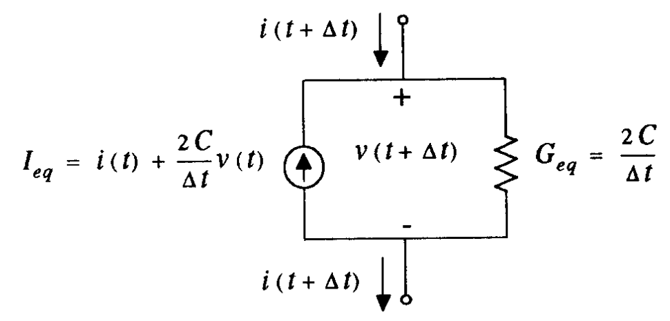
Thus \(v(t+\Delta t)\) can be solved by DC analysis.
For Nonlinear Circuit
Similarly, the nonlinear component will be linearized at \(v(t)\), and the capacitor will be convert to the circuits shown above. Then \(v(t+\Delta t)\) can be solved by DC analysis.