Reference
slides_an_introduction_to_digital_delta_sigma_modulators
paper a multiple modulator fractional divider
paper A Calibration-Free Fractional-N Analog PLL With Negligible DSM Quantization Noise
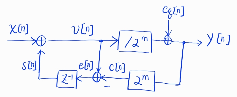
1st Order Error Feedback Modulator (EFM1)
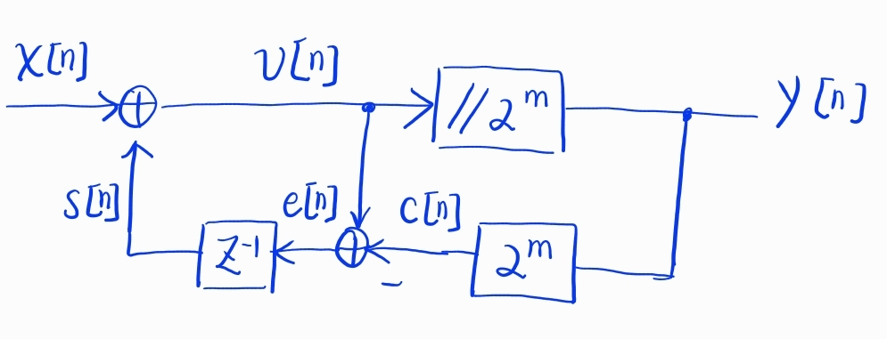
The dsim netlist example for \(m=10\)
1
2
3
4
5
6
7
8
9
10
11
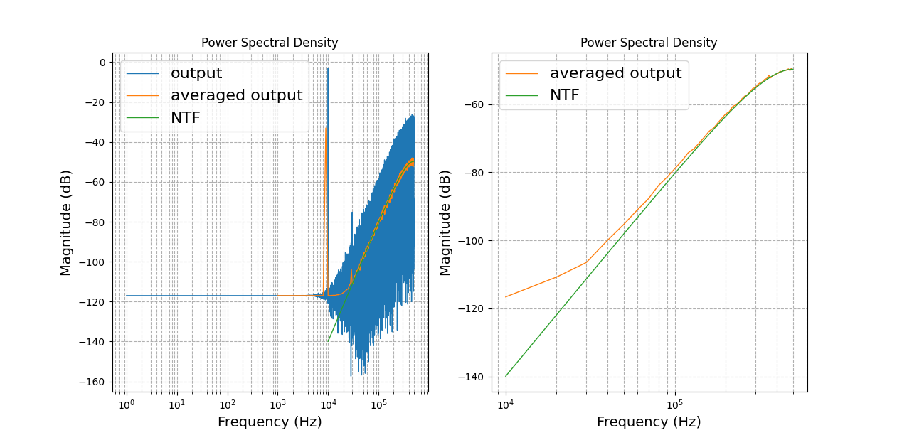
# 1st Order Error Feedback Modulator (EFM1)
# The output average should be input / 1024
--- Netlist
x, s --> add --> v
v, c --> sub --> e
e --> delay(1) --> s
y --> scaler(pow(2,10)) --> c
v --> integer_divide(pow(2,10)) --> y
--- Pin
in: x
out: e, y
The dsim maestro example for a single tone input
1
2
3
4
5
6
7
8
9
10
11
12
13
14
15
16
17
18
19
20
21
22
23
24
25
26
--- Test
dsim: /home/longhe/repos/dsim
schematic: efm1
runtime: y
runnum: 1000000
saveall: True
--- Parameters
x_mem = []
x = dsim.sig_init(lambda: lambda n: int(1024*1024*sin(0.02*n*pi)), x_mem)
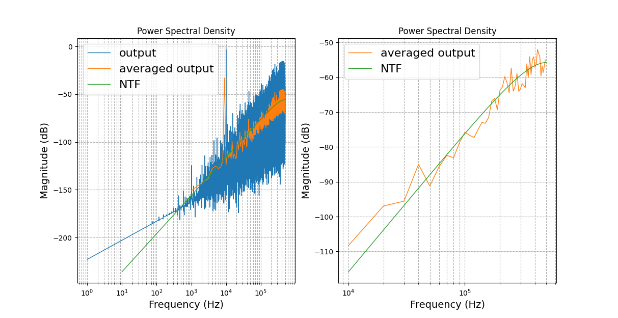
--- Plots
Fs = 1e6
ntf = lambda z: 1 - pow(z,-1)
S_n_out = lambda f: frac(1/12, Fs/2) * plot.tf2psd(ntf, var='z', Fs=Fs)(f)
fig, ax = plt.subplots(1,2)
plot.plot_psd(fig,ax[0],y_mem,Fs=Fs,color='C0',sumover_N=1,label='output')
plot.plot_psd(fig,ax[0],y_mem,Fs=Fs,color='C1',sumover_N=10000,label='averaged output')
plot.plot_psd(fig, ax[0], S_n_out, Fs=Fs, fstart = 1e3, fend=Fs/2,color='C2',label='NTF')
ax[0].legend(fontsize=16)
plot.plot_psd(fig,ax[1],y_mem,Fs=Fs,color='C1',sumover_N=10000,label='averaged output')
plot.plot_psd(fig, ax[1], S_n_out, Fs=Fs, fstart = 1e3, fend=Fs/2,color='C2',label='NTF')
ax[1].legend(fontsize=16)
ax[1].set_ylim(-100,-60)
ax[1].set_xlim(3e3,Fs/2)
plt.show()
the classical model of quantization (CMQ)
The \(e_q\) is assumed to be uniform distributed in \([-1/2,1/2]\), thus its variance
\[\int_{-1/2}^{1/2} x^2 dx = \dfrac{1}{12}\]also it is assumed to have flat psd in \([0, F_s/2]\). It can be calculated the NTF (noise transfer function) to the output \(y\) is
\[\begin{align} NTF(z) &= 1 - z^{-1} \end{align}\]Thus the output noise psd is
\[\begin{align} S_{n,out}(f) &= \dfrac{1}{12} \cdot \dfrac{1}{F_s/2} \cdot \vert 1 - e^{-j 2\pi f/Fs} \vert^2\\ &= \dfrac{1}{6} \cdot \dfrac{1}{Fs} \cdot \left( 1 - e^{-j 2\pi f/Fs} \right) \left( 1 - e^{j 2\pi f/Fs} \right)\\ &= \dfrac{1}{6} \cdot \dfrac{1}{Fs} \cdot e^{-j\pi f/Fs} \cdot \left( e^{j\pi f/Fs} - e^{-j \pi f/Fs} \right) \cdot e^{j \pi f/Fs} \cdot \left( e^{-j \pi f/Fs} - e^{j \pi f/Fs} \right)\\ &= \dfrac{1}{6} \cdot \dfrac{1}{Fs} \cdot 2 j \sin(\pi f/Fs) \cdot 2 j \sin(-\pi f/Fs)\\ &= \dfrac{1}{6 Fs} \cdot \left( 2 \sin\left(\dfrac{\pi f}{Fs}\right)\right)^2\\ & \approx \dfrac{1}{6} \cdot \dfrac{(2\pi f)^2}{F_s^3} \end{align}\]MASH
MASH stands for Multi-stAge noise SHaping.
MASH 1-1
The dsim netlist example for MASH 1-1
1
2
3
4
5
6
7
8
9
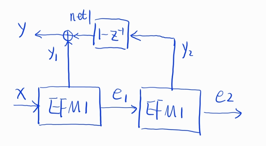
# MASH-1-1
--- Netlist
x --> efm1 --> e1, y1
e1 --> efm1 --> e2, y2
y2 --> tf([1,-1],[1,0],1) --> net1
y1, net1 --> add --> y
--- Pin
in: x
out: y
The dsim maestro exampel for MASH 1-1
1
2
3
4
5
6
7
8
9
10
11
12
13
14
15
16
17
18
19
20
21
22
23
24
--- Test
dsim: /home/longhe/repos/dsim
schematic: mash_1_1
runtime: y
runnum: 1000000
saveall: True
--- Parameters
x_mem = []
x = dsim.sig_init(lambda: lambda n: int(1024*sin(0.02*n*pi)), x_mem)
--- Plots
Fs = 1e6
ntf = lambda z: 1 - pow(z,-1)
S_n_out = lambda f: frac(1/12, Fs/2) * plot.tf2psd(ntf, var='z', Fs=Fs)(f)

fig, ax = plt.subplots(1,2)
plot.plot_psd(fig,ax[0],y_mem,Fs=Fs,color='C0',sumover_N=1,label='output')
ax[0].legend(fontsize=16)

plot.plot_psd(fig,ax[1],y_mem,Fs=Fs,color='C1',sumover_N=10000,label='averaged output')
plot.plot_psd(fig, ax[1], S_n_out, Fs=Fs, fstart = 1e3, fend=Fs/2,color='C2',label='NTF')
ax[1].legend(fontsize=16)
ax[1].set_ylim(-100,-60)
ax[1].set_xlim(3e3,Fs/2)
plt.show()
The four transfer function is EFM1 is
\[\begin{align} H_{x,y}(z) &= \dfrac{1}{2^m}\\ H_{e_q,y}(z) &= 1-z^{-1} \\ H_{x,e}(z) &= 0\\ H_{e_q,e} (z) &= - 2^m \end{align}\]The MASH 1-1 STF
\[\begin{align} y_1 &= \dfrac{1}{2^m} x\\ e_1 &= 0\\ y_2 &= 0\\ y &= \dfrac{1}{2^m} x \end{align}\]The MASH 1-1 NTF
\[\begin{align} y_1 &= (1-z^{-1}) e_{q1}\\ e_1 &= -2^m e_{q1}\\ y_2 &= \dfrac{1}{2^m} e_1 + (1-z^{-1}) e_{q2}\\ &= -e_{q1} + (1-z^{-1}) e_{q2}\\ y &= y_1 + (1-z^{-1})y_2\\ &= (1-z^{-1}) e_{q1} - (1-z^{-1}) e_{q1} + (1-z^{-1})^2 e_{q2}\\ &= (1-z^{-1})^2 e_{q2} \end{align}\]MASH 1-1-1

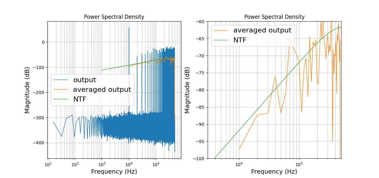
The dsim netlist example for MASH 1-1-1
1
2
3
4
5
6
7
8
9
10
11
12
# MASH-1-1-1
--- Netlist
x --> efm1 --> e1, y1
e1 --> efm1 --> e2, y2
e2 --> efm1 --> e3, y3
y3 --> diff --> net3
net3, y2 --> add --> net2
net2 --> diff --> net1
y1, net1 --> add --> y
--- Pin
in: x
out: y
The dsim maestro example for MASH 1-1-1
1
2
3
4
5
6
7
8
9
10
11
12
13
14
15
16
17
18
19
20
21
22
23
24
25
26
27
28
29
--- Test
dsim: /home/longhe/repos/dsim
schematic: mash_1_1_1
runtime: y
runnum: 1000000
save: x, y
--- Parameters
x_mem = []
x = dsim.sig_init(lambda: lambda n: int(1024*sin(0.02*n*pi)), x_mem)
--- Plots
Fs = 1e6
ntf = lambda z: pow(1 - pow(z,-1),3)
S_n_out = lambda f: frac(1/12, Fs/2) * plot.tf2psd(ntf, var='z', Fs=Fs)(f)

y_np = np.array(y_mem)
y_np = y_np - np.mean(y_mem)

fig, ax = plt.subplots(1,2)
plot.plot_psd(fig,ax[0],y_np.tolist(),Fs=Fs,color='C0',sumover_N=1,label='output')
plot.plot_psd(fig,ax[0],y_np.tolist(),Fs=Fs,color='C1',sumover_N=1000,label='averaged output')
plot.plot_psd(fig, ax[0], S_n_out, Fs=Fs, fstart = 1e4, fend=Fs/2,color='C2',label='NTF')
ax[0].legend(fontsize=16)

plot.plot_psd(fig,ax[1],y_np.tolist(),Fs=Fs,color='C1',sumover_N=10000,label='averaged output')
plot.plot_psd(fig, ax[1], S_n_out, Fs=Fs, fstart = 1e4, fend=Fs/2,color='C2',label='NTF')
ax[1].legend(fontsize=16)
# ax[1].set_ylim(-100,-60)
# ax[1].set_xlim(3e3,Fs/2)
plt.show()