From Dr. Chun-Yao Wang’ Lecture
Interesting Formula
\[\dfrac{1-x^N}{1-x} = 1 + x + x^2 + \dots + x^{N-1}\]gong bi ci fang jian yi, chu yi gong bi jian yi
\[\sum_{n=0}^{N-1} e^{jk(2\pi/N)n} = 0, \text{ when } k \ne 0, \pm N, \pm 2N, \dots\]First-Order First-Degree ODE
Integration by Parts
\[\int u dv = uv - \int vdu\]Ordinary, Partial, Order and Degree
Ordinary differential equation.
Partial differential equation.
Order of the differential equation.
Degree of the differential equation.
Linear differential equation.
General solution.
Particular solution.
Singular solution.
\[y'=f(x,y)\]or
\[M(x,y)dx + N(x,y)dy = 0\]Direct Integral
Seperable Equation
Seperable After Changing Variable
- First-Order First-Degree Homogeneous ODE, \(y'=f(y/x)\)
- \((a_1 x + b_1 y + c_1)dx + (a_2 x +b_2 y + c2)dy = 0\)
- \(y'=f(ax+by+c)\)
Exact Differential Equations
\[\begin{align} & M(x,y)dx + N(x,y)dy = 0\\ & \dfrac{\partial M}{\partial y} = \dfrac{\partial N}{\partial x} \end{align}\]Integrating Factors
\[I(x,y)M(x,y)dx + I(x,y)N(x,y)dy = 0 \quad \text{ is exact differential equation}\] \[I(x) = \exp(\int \dfrac{\dfrac{\partial M}{\partial y} - \dfrac{\partial N}{\partial x}}{N} dx )\] \[I(y) = \exp(\int \dfrac{\dfrac{\partial M}{\partial y} - \dfrac{\partial N}{\partial x}}{-M} dy )\] \[I(x+y) = \exp(\int \dfrac{\dfrac{\partial M}{\partial y} - \dfrac{\partial N}{\partial x}}{N-M} d(x+y))\] \[I(xy) = \exp(\int \dfrac{\dfrac{\partial M}{\partial y} - \dfrac{\partial N}{\partial x}}{Ny-Mx} d(xy))\] \[I(x-y) = \exp(\int \dfrac{\dfrac{\partial M}{\partial y} - \dfrac{\partial N}{\partial x}}{N+M} d(x+y))\]First Order Linear ODE
\[y'+P(x)y = Q(x)\] \[I(x) = \exp(\int P(x)dx)\] \[y = \dfrac{1}{I(x)} \int Q(x) I(x) dx + \dfrac{C}{I(x)}\]Linearized ODE
- Bernoulli Equation: \(y' + P(x)y = Q(x) \cdot y^n\). Let \(u=y^{1-n}\)
- \(\dfrac{dv}{dy}y' + P(x)v(y)=Q(x)\)
- Riccati Equation: \(y'=P(x)y^2 + Q(x)y + R(x)\)
Linear ODE
We concentrate on linear ODE
\[y'' + p(x)y' + q(x)y = f(x)\]If \(f(x)=0\), we call it homogeneous equation. Otherwise non-homogeneous equation.
Linear ODE Theory
Homogeneous Equation
- Theorem 2.2:
Let \(y_1(x)\) and \(y_2(x)\) be solutoins of \(y''+p(x)y'+q(x)y = 0\). Then any linear combination of these solutions, e.g., \(c_1 y_1(x) + c_2 y_2(x)\), is also a solutoin.
- Definition 2.1: Linear Dependence/Independence
only when
\[c_1 = c_2 = \dots = 0\]- Wronskian
If \(W(x) = 0\), they are linear dependent. Otherwise L.I. The Wronskian also apply for more than two functions.
\[\begin{equation} W(x) = \left|\begin{array}{rr} y_1 & y_2 & y_3\\ y_1' & y_2' & y_3'\\ y_1'' & y_2'' & y_3'' \end{array}\right| \end{equation}\]- Abel’s Identity
\(y_1, y_2\) are solutions. Then
\[W(x) = C \cdot \exp(-\int P(x)dx)\]- Theorem 2.4 (YouTube 8C):
Let \(y_1, y_2\) be linearly independent solutions of \(y'' + P(x)y' + Q(x)y = 0\). Then every solution is a linear combination of \(y_1\) and \(y_2\).
\[y'' + p(x)y' + q(x)y = 0\]with initial conditon \(y(x_0)=A, y'(x_0)=B\)
\[y = C_1 y_1 + C_2 y_2\]Cramer’s rule
\[\begin{bmatrix} y_1(x_0) & y_2(x_0)\\ y_1'(x_0) & y_2'(x_0) \end{bmatrix} \begin{bmatrix} C_1\\ C_2 \end{bmatrix}= \begin{bmatrix} A\\ B \end{bmatrix}\] \[\begin{equation} C_1 = \dfrac{1}{W(x_0)} \left|\begin{array}{rr} A & y_2(x_0)\\ B & y_2'(x_0)\\ \end{array}\right| \end{equation}\] \[\begin{equation} C_2 = \dfrac{1}{W(x_0)} \left|\begin{array}{rr} y_1(x_0) & A\\ y_1'(x_0) & B\\ \end{array}\right| \end{equation}\]Nonhomogeneous Equation
\[y''+p(x) + q(x)y = f(x)\]Theorem 2.5:
\(y_1, y_2\) is linearly independent solutions for \(y''+p(x)y'+q(x)y=0\). If \(y_p\) is solution for the nonhomogeneous equation, then any solution can be given by
\[c_1 y_1 + c_2 y_2 + y_p\]Linear Constant Coefficient ODE
\[y'' + a_1 y' + a_0 y =R(x)\]Homogeneous Solutions
\[\lambda^2 + a_1 \lambda + a_0 = 0\] \[\lambda = \dfrac{-a_1 \pm \sqrt{a_1^2 - 4a_0}}{2}\]Case 1: \(a_1^2 - 4a_0 > 0\)
\[\begin{align} \lambda_1 &= \dfrac{-a_1 + \sqrt{a_1^2 - 4a_0}}{2}\\ \lambda_2 &= \dfrac{-a_1 - \sqrt{a_1^2 - 4a_0}}{2} \end{align}\] \[y_h(x) = C_1 \exp(\lambda_1 x) + C_2 \exp(\lambda_2 x)\]Case 2: \(a_1^2 - 4a_0 = 0\)
\[\begin{align} \lambda &= \dfrac{-a_1}{2} \end{align}\] \[y_h(x) = C_1 \exp(\lambda x) + C_2 x\exp(\lambda x)\]Case 3: \(a_1^2 - 4a_0 < 0\)
\[\lambda = \alpha \pm i\beta\] \[y_h(x) = C_1 \exp(\alpha x) \cos(\beta x) + C_2 \exp(\alpha x) \sin(\beta x)\]Method of Undetermined Coefficient
\[y^{(n)} + a_{n-1} y^{(n-1)} + \dots + a_1 y^{(1)} + a_0 y =R(x)\]| \(R(x)\) | \(y_p(x)\) |
|---|---|
| \(R_1(x)+R_2(x)\) | \(y_{p1}(x)+y_{p2}(x)\) |
| \(k\) | \(A\) |
| \(e^{ax}\) | \(Ae^{ax}\) |
| \(\cos ax\) | \(A\cos ax + B\sin ax\) |
| \(\sin ax\) | \(A\cos ax + B\sin ax\) |
| \(a_n x^n + \dots + a_1 x + a_0\) | \(A_n x^n + \dots + A_1 x + A_0\) |
| \(e^{ax}\cos bx \quad\) or \(\quad e^{ax}\sin bx\) | \(e^{ax}(A\cos bx + B\sin bx)\) |
| \(e^{ax}(a_n x^n + \dots + a_1 x + a_0)\) | \(e^{ax}(A_n x^n + \dots + A_1 x + A_0)\) |
| \(\cos bx (a_n x^n + \dots + a_1 x + a_0)\) | \((A_n x^n + \dots + A_0)\cos bx + (B_n x^n + \dots + B_0)\sin bx\) |
| \(e^{ax} \cos bx (a_n x^n + \dots + a_0)\) | \(e^{ax}(A_n x^n + \dots + A_0)\cos bx + e^{ax}(B_n x^n + \dots + B_0)\sin bx\) |
Theorem: If the \(y_p(x)\) in the table is in the homogeneous solution, we should use \(x^m y_p(x)\), where \(m\) is the minimum positive integer such that \(x^m y_p(x)\) is not in the homogeneous solution. This claim can be proved by the method of variation of parameters.
Method of Variation Parameter
\[y'' + a_1(x)y' + a_0(x)y = R(x)\] \[y_h(x) = C_1 y_1(x) + C_2 y_2(x)\] \[y_p(x) = \phi_1(x)y_1(x) + \phi_2(x)y_2(x)\] \[\begin{bmatrix} y_1 & y_2\\ y_1' & y_2' \end{bmatrix} \begin{bmatrix} \phi_1'\\ \phi_2' \end{bmatrix} =\begin{bmatrix} 0\\ R(x) \end{bmatrix}\] \[\phi_1(x) = \int \dfrac{-R(x)y_2(x)}{W(y_1,y_2)}dx\] \[\phi_2(x) = \int \dfrac{R(x)y_1(x)}{W(y_1,y_2)}dx\]If third order
\[\begin{bmatrix} y_1 & y_2 & y_3\\ y_1' & y_2' & y_3'\\ y_1'' & y_2'' & y_3'' \end{bmatrix} \begin{bmatrix} \phi_1'\\ \phi_2'\\ \phi_3' \end{bmatrix} =\begin{bmatrix} 0\\ 0\\ R(x) \end{bmatrix}\]Cauchy-Euler Equation
\[a_n x^n y^{(n)} + \dots + a_1 x y^{(1)} + a_0 y = R(x)\]Let \(x = \exp(u)\), \(u = \ln x\) , \(D_u = \dfrac{d}{du}\)
\[x^n \dfrac{d^n y}{dx^n} = x^n (D_x)^n y = D_u (D_u - 1) (D_u - 2) \dots (D_u - n + 1)y\]Legendre ODE
\[a_n (bx + c)^n y^{(n)} + \dots + a_1 (bx+c) y^{(1)} + a_0 y = R(x)\]Let \(z = bx + c\)
\[\dfrac{d^n y}{dx^n} = b^{n} \dfrac{d^n y}{dz^n}\]Reduction of Order (13A)
\[y'' + P(x)y' + Q(x)y = R(x)\]if \(u(x)\) is a homogenuous solution
\[u'' + P(x)u' + Q(x)u = 0\]Let
\[y(x) = u(x)v(x)\]System of Linear ODEs
A linear first-order system of \(n\) equations in the \(n\) unknowns \(x_1(t),\dots,x_n(t)\) is of the form
\[\begin{align} a_{11}(t) x_1' + \dots + a_{1n}(t)x_n' + b_{11}(t) x_1 + \dots + b_{1n}(t) x_n &= f_1(t)\\ &\vdots\\ a_{n1}(t) x_1' + \dots + a_{nn}(t)x_n' + b_{n1}(t) x_1 + \dots + b_{nn}(t) x_n &= f_n(t)\\ \end{align}\]A linear second-order system will be similar.
Laplace Transform
The Laplace Transform
\[F(s) = \int_{0}^{\infty} f(t)e^{-st}dt\]The Laplace transform table
| \(f(t)\) | \(F(s)\) | Notes |
|---|---|---|
| \(t^{n}\) | \(\dfrac{n!}{s^{n+1}}\) | \(n = 0,1,2,3,\dots\) |
| \(e^{at}\) | \(\dfrac{1}{s-a}\) | |
| \(\sin(at)\) | \(\dfrac{a}{s^2+a^2}\) | |
| \(\cos(at)\) | \(\dfrac{s}{s^2+a^2}\) | |
| \(\delta(t)\) | \(1\) |
The inverse Laplace transform table
| \(F(s)\) | \(f(t)\) | Notes |
|---|---|---|
| \(\dfrac{1}{s^{n+1}}\) | \(\dfrac{t^n}{n!}\) | \(n = 0,1,2,3,\dots\) |
| \(\dfrac{1}{s-a}\) | \(e^{at}\) | |
| \(\dfrac{1}{s^2+a^2}\) | \(\dfrac{1}{a}\sin(at)\) | |
| \(\dfrac{s}{s^2+a^2}\) | \(\cos(at)\) |
Heaviside Expansion
\[F(s) = \dfrac{P(s)}{Q(s)}\]Assume \(P(s), Q(s)\) are real polynomials, they have no common factors, and the order of \(Q(s)\) is higher than \(P(s)\).
Case 1: \(Q(s)=0\) has \(n\) distinct roots.
\[\dfrac{P(s)}{Q(s)} = \dfrac{A_1}{s-a_1} + \dfrac{A_2}{s-a_2} + \dots + \dfrac{A_n}{s-a_n}\] \[A_k = \dfrac{P(s)}{Q(s)} \cdot (s-a_k)\]Case 2: \(Q(s)=0\) has repeated roots, e.g., \(m\)-repeated \(a_k\).
\[\dfrac{P(s)}{Q(s)} = \dfrac{A_1}{s-a_1} + \dots + \dfrac{C_m}{(s-a_k)^m} + \dfrac{C_{m-1}}{(s-a_k)^{m-1}} + \dots \dfrac{C_1}{s-a_k} + \dots\] \[C_m = \lim_{s\to a_k} [\dfrac{P(s)}{Q(s)} (s-a_k)^m ]\] \[C_{m-1} = \lim_{s\to a_k} \{ \dfrac{d}{ds}[\dfrac{P(s)}{Q(s)} (s-a_k)^m]\}\] \[C_{m-1} = \dfrac{1}{2!} \lim_{s\to a_k} \{ \dfrac{d^2}{ds^2}[\dfrac{P(s)}{Q(s)} (s-a_k)^m]\}\]Case 3: complex conjugate roots
\[\dfrac{As + B}{(s-a)^2+b^2}\] \[\lim_{s\to a+b j} \{\dfrac{P(s)}{Q(s)}[(s-a)^2+b^2]\} = A(a+bj) + B\]Solution of Initial Value Problems
\[\mathscr{L}\{f^{(n)}(t)\} = s^n F(s) - s^{n-1} f(0) - s^{n-2}f'(0) - \dots - f^{(n-1)}(0)\]If all initial value are zero, then the Laplace transform of the impulse response can be easily calculated as \(H(s)\). Also, the value \(H(j\omega)\) is very meanful. First
\[H(j\omega) = \int_{-\infty}^{\infty} h(t)e^{-j\omega t} dt, \quad \text{(because h(t) = 0 when t is less than 0)}\]which is the Fourier transform of the impulse response. Secondly, if the input is \(e^{j\omega t}\) (for \(t > 0\)), and all inital condition is still zero.
\[y(t) = \int_{0}^{t} h(\tau) e^{j\omega (t-\tau)} d\tau = e^{j\omega t} \int_{0}^{t} h(\tau) e^{-j\omega \tau} d\tau\]Thus, the response will approach to \(H(j\omega) e^{j\omega t}\) when \(t \to \infty\).
ODE with Polynomial Coefficients
\[\mathscr{L}\{t^n f(t)\} = (-1)^n\dfrac{d^n F(s)}{ds^n}\]Systems of Linear ODEs
20E
Series Solutions
Power Series
Definition 4.4 (Power Series):
\[\sum_{n=0}^{\infty} a_n (x-x_0)^n\]It is obvious it converges at \(x = x_0\).
Theorem 4.5:
If the power series converge at \(x_1\), then it converges absolutely for all \(x\) such that \(\vert x-x_0 \vert < \vert x_1 - x_0\vert\).
Theorem:
There are three possibilities:
- It converges only at \(x_0\).
- It converges in a finite interval, the endpoints may or may not converge. \((x_0-r, x_0+r)\) is called the open interval of the convergence.
- It converges in \(\mathbb{R}\).
Theorem 4.6:
For series \(\sum_{0}^{\infty} b_n\), where \(b_n \ne 0\) for all \(n\). Then if \(\lim_{n\to\infty} \vert \dfrac{b_{n+1}}{b_n} \vert = L\) exists,
- if \(L < 1\), then the series converges absolutely.
- if \(L = 1\), no conclusion.
- if \(L > 1\), the series diverges.
Taylor Series:
\[\sum_{n=0}^{\infty} \dfrac{1}{n!}f^{(n)}(x_0)(x-x_0)^n\]Definition 4.1 (Analytic Function):
A function \(f\) is analytic at \(x_0\) if \(f(x)\) has a power series representation
\[f(x) = \sum_{n=0}^{\infty} a_n (x-x_0)^n\]in a non-zero interval \((x_0-r, x_0+r)\).
Solution of IVP (21E)
Theorem 4.1:
Let \(p\) and \(q\) be analytic at \(x_0\). Then the initial value problem
\[y' + p(x)y + q(x); \quad y(x_0) = y_0\]has a solution that is analytic at \(x_0\).
Theorem 4.2:
Let \(p, q\) and \(f\) be analytic at \(x_0\). Then the initial value problem
\[y'' + p(x)y' + q(x)y = f(x); \quad y(x_0)=A, y'(x_0) = B\]has a unique solution that is also analytic at \(x_0\).
Recurrence Relations (22B)
match of terms
Singular Points (23A)
- Ordinary point:
\(x_0\) is an ordinary point of equation
\[P(x)y'' + Q(x)y' + R(x)y = F(x)\]if \(P(x_0) \ne 0\) and \(Q(x)/P(x), R(x)/P(x)\) and \(F(x)/P(x)\) are analytic at \(x_0\).
- Singular point:
If it is not ordinary point, it is singular point.
- Regular singular point:
\(x_0\) is a regular singular point of equation
\[P(x)y'' + Q(x)y' + R(x)y = 0\]if \(x_0\) is a singular point, and \((x-x_0)\dfrac{Q(x)}{P(x)}\) and \((x-x_0)^2\dfrac{R(x)}{P(x)}\) are analytic at \(x_0\).
- Irregular singular point:
A singular point that is not regular is said to be an irregular singular point.
Frobenius Series (23C)
\[y'' + \dfrac{p(x)}{x}y' + \dfrac{q(x)}{x^2} y = 0\] \[F(r) = r(r-1) + p_0 r + q_0 = 0\] \[\begin{align} F(r+m) c_m &= \left[(m+r)(m+r-1) + (m+r)p_0 + q_0\right] c_m\\ &= -\sum_{k=0}^{m-1} \left[(k+r)p_{m-k} + q_{m-k}\right] c_k, \quad m \ge 1 \end{align}\]- If \(r_1 - r_2\) is not an (positive or negative or zero) integer.
- If \(r_1 - r_2 = 0\)
where
\[d_m = \left( \dfrac{\partial c_m}{\partial r}\right)_{r=r_1}, \quad m \ge 1\]The book Ordinary Differential Equations, Chapter 36 well explains why the formula takes the absolute value. It is just meant to maintain the function to be real value when \(x<x_0\). If we only consider \(x>x_0\), the absolute value is useless. Also, if \(r\) is a integer number, the absolute value is not necessary.
Special Function
\[y(x) = \sum_{m=0}^{\infty} C_m x^m\]Hermite Polynomials
\[y'' - 2x y' + 2ny = 0\] \[C_m = \dfrac{2(m-2-n)}{m(m-1)}C_{m-2}, \quad m\ge 2\] \[y(x) = A_1 y_1(x) + A_2 y_2(x)\]if \(n\) is some nonnegative integer (\(n \ge 0\)), then one of the solution is a polynomial (with finite terms).
Fourier Series
Fourier Series
If function \(f(t)\) has period \(T\), then \(\omega = 2\pi/T\)
\[f(t) \sim A_0 + \sum_{n=1}^{\infty} A_n \sin(n\omega t + \varphi_n)\]or
\[\begin{align} f(t) &\sim \dfrac{a_0}{2} + \sum_{n=1}^{\infty} [a_n \cos(n\omega t) + b_n \sin(n\omega t)]\\ a_0 &= 2A_0 = \dfrac{2}{T} \int_T f(t)dt\\ a_n &= A_n \sin\varphi_n = \dfrac{2}{T} \int_T f(t)\cos(n\omega t)dt\\ b_n &= A_n \cos\varphi_n = \dfrac{2}{T} \int_T f(t)\sin(n\omega t)dt \end{align}\]or
\[f(t) \sim \sum_{n=-\infty}^{\infty} c_n e^{j n \omega t}\] \[c_n = \dfrac{1}{T}\int_T f(t) e^{-j n \omega t} dt\]Examples
- Impulse Train
- Odd function square wave
- Even function square wave
Convergence (25C)
Fourier Transform
\[F(\omega) = \int_{-\infty}^{\infty} f(t) \exp(-j\omega t) dt\] \[f(t) = \dfrac{1}{2\pi} \int_{-\infty}^{\infty} F(\omega) \exp(j\omega t) d\omega\]Examples
- Convolution theorem
- FT of multiplication
- Time scaling
- Frequency scaling
- finite unit step
- comb function (impulse train)
- Ideal low pass
If the bandwidth is \(\omega_b\), \(\mathrm{RECT}\left(\dfrac{\omega}{2\omega_b}\right)\)
\[f(t) = \dfrac{\omega_b}{\pi} \mathrm{sinc}\left(\dfrac{\omega_b t}{\pi}\right)\]Multi-Variable Functions
From Prof. Yen’s Lecture
Partial Derivatives
For function \(f(x,y)\)
\[f_{xy} = \dfrac{\partial}{\partial y} \Big(\dfrac{\partial f}{\partial x}\Big) = \dfrac{\partial^2 f}{\partial y \partial x}\]Theorem (Equalty of Derivatives): if \(f_x, f_y, f_{xy}, f_{yx}\) are all continuous in some neighborhood of \((x_0,y_0)\), then \(f_{xy}=f_{yx}\).
We say \(f\) is \(C^n\) if all of the partial derivatives of \(f\), through \(n\)th order, are continuous. For example, \(f\) is \(C^2\) in \(\mathbb{R}\) if \(f_x, f_y, f_{xx}, f_{xy}, f_{yy}\) are continuous in \(\mathbb{R}\).
Chain Rule
For function \(f(x(t),y(t)) = R(t)\)
\[\dfrac{d R}{dt} = \dfrac{\partial f}{\partial x} \dfrac{d x}{dt} + \dfrac{\partial f}{\partial y} \dfrac{d y}{dt}\]For function \(f(u,v) = f(u(x,y), v(x,y)) = F(x,y)\)
\[\dfrac{\partial F}{\partial x} = \dfrac{\partial f}{\partial u} \dfrac{\partial u}{\partial x} + \dfrac{\partial f}{\partial v} \dfrac{\partial v}{\partial x}\]Comments: we have to use a different symbol (e.g., \(R\) or \(F\)) for the composite function, otherwise it is very easy to make mistakes.
Taylor’s Formula
For single variable function
\[\begin{align} f(x) &= f(a) + \dfrac{f'(a)}{1!}(x-a) + \dfrac{f''(a)}{2!}(x-a)^2 + \dots + \dfrac{f^{(n-1)}(a)}{(n-1)!}(x-a)^{n-1} + \dfrac{f^{(n)}(\xi)}{n!}(x-a)^n \end{align}\]For multi-variable function
\[f(x_0,y_0) = f(a,b) + \dfrac{1}{1!}D f\vert_{a,b} + \dots + \dfrac{1}{(n-1)!} D^{n-1} f\vert_{a,b} + \dfrac{1}{n!}D^n f\vert_{\xi,\eta}\] \[D = (x_0-a)\dfrac{\partial}{\partial x} + (y_0-b)\dfrac{\partial}{\partial y}\] \[Df = (x_0-a)f_x + (y_0-b)f_y\] \[D^2 f = (x_0-a)^2f_{xx} + 2(x_0-a)(y_0-b)f_{xy} + (y_0-b)^2 f_{yy}\]or if it doesn’t cause confusion
\[f(x,y)=f(x_0,y_0) + f_x(x-x_0) + f_y(y-y_0) + \dfrac{1}{2!}[f_{xx}(x-x_0)^2 + 2f_{xy}(x-x_0)(y-y_0) + f_{yy}(y-y_0)^2]\]Mean Value Theorem
For single variable function
\[f(x) = f(a) + f'(\xi)(x-a)\]For multi-variable function
\[f(x,y) = f(a,b) + (x-a)f_x(\xi,\eta) + (y-b)f_y(\xi,\eta)\]Implicit Function
For explicit function \(y=y(x)\), its implicit function counterpart is \(f(x,y)=0\).
Theorem: For implicit function \(f(x,y)=0\), if it has explicit function \(y=y(x)\), then the corresponding \(y'=-f_x/f_y\).
Theorem (Implicit Function Theorem): Let \(f(x,y)=0\) be satisfied by a pair of real numbers \(x_0, y_0\) so that \(f(x_0,y_0)=0\), and suppose that \(f(x,y)\) is \(C^1\) in some neighborhood of \((x_0,y_0)\) with
\[\dfrac{\partial f}{\partial y}(x_0,y_0) \ne 0\]Then \(f(x,y)=0\) uniquely implies a function \(y(x)\) in some neighborhood \(N\) of \(x_0\) such that \(y(x_0)=y_0\), where \(y(x)\) is differentiable in \(N\).
Define: Jacobian
\[\dfrac{\partial(f,g)}{\partial(u,v)}= \begin{vmatrix} f_u & f_v\\ g_u & g_v \end{vmatrix}\]Theorem: For implicit function
\[\begin{cases} f(x, y; u, v)=0\\ g(x, y; u, v)=0 \end{cases}\]the correspond explicit function
\[\begin{cases} u=u(x,y)\\ v=v(x,y) \end{cases}\]the derivatives \(u_x,u_y,v_x,v_y\) can be found by
\[\begin{bmatrix} f_u & f_v\\ g_u & g_v \end{bmatrix} \begin{bmatrix} u_x\\ v_x \end{bmatrix} =\begin{bmatrix} -f_x\\ -g_x \end{bmatrix}\] \[\begin{bmatrix} f_u & f_v\\ g_u & g_v \end{bmatrix} \begin{bmatrix} u_y\\ v_y \end{bmatrix} =\begin{bmatrix} -f_y\\ -g_y \end{bmatrix}\] \[u_x = -\dfrac{\dfrac{\partial(f,g)}{\partial(x,v)}}{\dfrac{\partial(f,g)}{\partial(u,v)}}, \quad u_y = -\dfrac{\dfrac{\partial(f,g)}{\partial(y,v)}}{\dfrac{\partial(f,g)}{\partial(u,v)}}, \quad v_x = -\dfrac{\dfrac{\partial(f,g)}{\partial(u,x)}}{\dfrac{\partial(f,g)}{\partial(u,v)}}, \quad v_y = -\dfrac{\dfrac{\partial(f,g)}{\partial(u,y)}}{\dfrac{\partial(f,g)}{\partial(u,v)}}\]For general implicit functions
\[\begin{align} g_1(x_1,\dots,x_m;y_1,\dots,y_n)=0\\ \vdots\\ g_n(x_1,\dots,x_m;y_1,\dots,y_n)=0 \end{align}\]the derivatives can be calculated as
\[\dfrac{\partial y_j}{\partial x_k} = -\dfrac{J(y_1,\dots,y_{j-1},x_k,y_{j+1},\dots,y_n)}{J(y_1,\dots,y_n)}\]Jacobian Matrix
Theorem: For functions
\[\begin{align} u_1&=u_1(x_1,\dots,x_n)\\ &\dots\\ u_n&=u_n(x_1,\dots,x_n) \end{align}\]and its correspond implicit function
\[\begin{align} x_1&=x_1(u_1,\dots,u_n)\\ &\dots\\ x_n&=x_n(u_1,\dots,u_n) \end{align}\]then the multiplication of two Jacobian matrix
\[\dfrac{\partial(u_1,\dots,u_n)}{\partial(x_1,\dots,x_n)} \dfrac{\partial(x_1,\dots,x_n)}{\partial(u_1,\dots,u_n)} = I\]then their determinant has multiplication \(1\).
PDE Example
\[\begin{align} x &= r\cos\theta\\ y &= r\sin\theta \end{align}\] \[\dfrac{\partial r}{\partial x} = \cos\theta, \quad \dfrac{\partial r}{\partial y} = \sin\theta\] \[\dfrac{\partial \theta}{\partial x} = -\dfrac{\sin\theta}{r}, \quad \dfrac{\partial \theta}{\partial y} = \dfrac{\cos\theta}{r}\] \[T_{xx} + T_{yy} = 0\]in polar coordinates
\[T(x(r,\theta),y(r,\theta)) = U(r,\theta)\] \[? \quad U_{rr} + \dfrac{1}{r}U_r + \dfrac{1}{r^2} U_{\theta \theta} = 0\]in spherical coordinates
Maximum And Minimum
From the Taylor’s formula, if all the first order partial derivatives are zero, and the second derivatives matrix is positive (or negative) definite, then the function is at maximum (or minimum).
\[f(x_1,y_1)\]the necessary condition for it is at maximum or minimum
\[f_{x_1} = f_{x_2} = 0\]if its second derivatives matrix is positive definite, it is at minimum point
\[\begin{pmatrix} f_{x_1 x_1} & f_{x_1 x_2}\\ f_{x_2 x_1} & f_{x_2 x_2} \end{pmatrix}\]Constrained Extrema
We want to find extrema for
\[f(x_1,x_2,\dots,x_n)\]under the conditions
\[\begin{align} g_1(x_1,x_2,\dots,x_n) = 0\\ \vdots\\ g_k(x_1,x_2,\dots,x_n) = 0 \end{align}\]Then we need to find the extrema for function
\[F(x_1,\dots,x_{n-k}) = f\left(x_1,\dots,x_{n-k},x_{n-k+1}\left(x_1,\dots,x_{n-k}\right),\dots,x_n\left(x_1,\dots,x_{n-k}\right)\right)\]if the functions \(x_{n-k+1}(), \dots\) are easy to calculate, this method is easy and straightforward.
Lagrange Method
\[f^{*} = f + \lambda_1 g_1 + \dots + \lambda_k g_k\]The necessary condition for extrema is
\[\begin{align} f_{x_1} + \lambda_1 g_{1_{x_1}} + \dots + \lambda_k g_{k_{x_1}} = 0\\ \vdots\\ f_{x_n} + \lambda_1 g_{1_{x_n}} + \dots + \lambda_k g_{k_{x_n}} = 0 \end{align}\]then we can solve
\[\begin{align} x_1 = x_1(\lambda_1,\dots,\lambda_k)\\ \vdots\\ x_n = x_n(\lambda_1,\dots,\lambda_k) \end{align}\]then using the equations \(g_1,\dots,g_k\), we can get the values of \(\lambda_1,\dots,\lambda_k\).
Famous examples including:
- Fermat’s principle of least time.
Leibniz Rule
\[I(t) = \int_{a(t)}^{b(t)} f(x,t)dx\] \[I'(t) = \int_{a}^{b}\dfrac{\partial f}{\partial t}dx + b' f(b,t) - a'f(a,t)\]3D Vectors
Dot Product
\[\vec{u}\cdot\vec{v} = \left\vert\vec{u}\right\vert \left\vert\vec{u}\right\vert \cos\theta, \quad 0 \le \theta \le \pi\]It is projection.
\[\vec{u}\cdot\vec{v} = \vec{v}\cdot\vec{u}\]Cross Product
\[\vec{u}\times\vec{v} = \left\vert\vec{u}\right\vert \left\vert\vec{v}\right\vert \sin\theta \,\,\vec{e} , \quad 0 \le \theta \le \pi, \quad \text{right-hand rule}\]It is the area of parallelogram.
\[\vec{u}\times\vec{v} = -\vec{v}\times\vec{u}\]Cartesian Coordinates
\[\vec{u}=u_i\, \hat{i} + u_j\,\hat{j} + u_k\,\hat{k}\]where \(\hat{i},\hat{j},\hat{k}\) are orthonormal basis.
\[\hat{i}\times\hat{j}=\hat{k}, \quad \hat{j}\times\hat{k}=\hat{i}, \quad \hat{k}\times\hat{i}=\hat{j}\] \[\vec{u}\times\vec{v}= \begin{vmatrix} \hat{i} & \hat{j} & \hat{k}\\ u_i & u_j & u_k\\ v_i & v_j & v_k \end{vmatrix}\] \[\begin{align} &\vec{u}\times \vec{v} = \vert u \vert \vert v\vert \sin\theta\\ =& \vert u\vert\vert v\vert \sqrt{1-\cos^2\theta}\\ =& \sqrt{\vert u\vert^2 \vert v\vert^2 - (\vec{u}\cdot\vec{v})^2} \end{align}\]Multuple Products
\[\vec{u}\cdot\left(\vec{v}\times\vec{w}\right)=\vec{u}\cdot\vec{v}\times\vec{w}= \begin{vmatrix} u_1 & u_2 & u_3\\ v_1 & v_2 & v_3\\ w_1 & w_2 & w_3 \end{vmatrix}=\vec{u}\times\vec{v}\cdot\vec{w}\]\(\left\vert \vec{u}\cdot\vec{v}\times\vec{w}\right\vert\) is the volume of the parallelepiped.
\[\vec{u}\times\left(\vec{v}\times\vec{w}\right) = \left(\vec{u}\cdot\vec{w}\right)\vec{v} - \left(\vec{u}\cdot\vec{v}\right) \vec{w}\]Differentiation
\[\dfrac{d}{dt}\left( \vec{u} \cdot \vec{v} \right) = \dot{\vec{u}} \cdot \vec{v} + \vec{u} \cdot \dot{\vec{v}}\]Coordinates
\[\begin{align} \vec{R}(t) &= x(t)\hat{i} + y(t)\hat{j} + z(t)\hat{k}, \quad \text{in cartesian coordinate}\\ &= r(t)\hat{e_r} + \theta(t)\hat{e_{\theta}} + z(t)\hat{k}, \quad \text{in cylindrical coordinate}\\ &= \rho(t)\hat{e_{\rho}} + \phi(t)\hat{e_\phi} + \theta(t)\hat{e_{\theta}}, \quad \text{in spherical coordinate} \end{align}\] \[\vec{R}'(t) = x'(t)\hat{i} + y'(t)\hat{j} + z'(t)\hat{k}\]\(\vec{R}'(t)\) is at the tagent direction of the curve.
\[\text{if } \vert R(t)\vert \text{ is constant}, \vec{R}(t) \cdot \vec{R}'(t) = 0\]Polar Coordinates
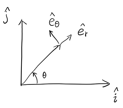
Cylindrical Coordinates
\[\hat{e_r} \times \hat{e_\theta} = \hat{e_z}\] \[\vec{R}(t) = r \hat{e_r} + z \hat{e_z}\] \[\vec{R}'(t) = \dot{r} \hat{e_r} + r \dot{\theta} \hat{e_\theta} + \dot{z} \hat{e_z}\] \[\vec{R}''(t) = (\ddot{r} - r\dot{\theta}^2) \hat{e_r} + (2 \dot{r}\dot{\theta} + r\ddot{\theta}) \hat{e_\theta} + \ddot{z} \hat{e_z}\]Spherical Coordinates
\[\hat{e_\rho} \times \hat{e_\phi} = \hat{e_\theta}\]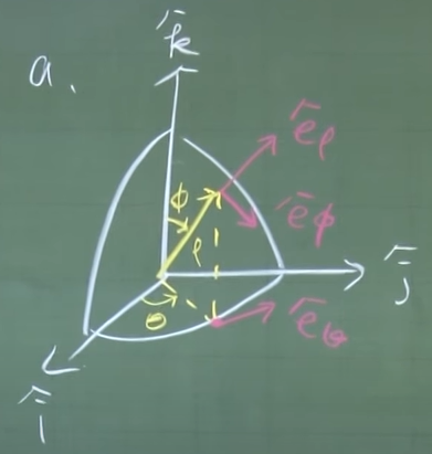
Omega Method (4B,TBD)
Curves, Surfaces, and Volumes
Line Integral
Arc Length
A curve can be described by position vector
\[\vec{R}(\tau) = x(\tau)\hat{i} + y(\tau)\hat{j} + z(\tau)\hat{k}\]Terms
- Closed curve.
- Simple curve.
- Continuous.
- Smooth.
Length of a curve
\[S = \int ds = \int_a^b \sqrt{\vec{R'}\cdot \vec{R'}} d\tau\]Line Integral
\[\int_c f(x,y,z) ds = \int_c f(x(\tau),y(\tau),z(\tau)) \sqrt{\vec{R'}\cdot \vec{R'}} d\tau\] \[\int_c (\alpha f + \beta g) ds = \alpha\int_c f ds + \beta\int_c g ds\] \[\oint\]Surface Integral
Double Integral
If we are doing double integral in \(x,y\) axis
\[\int\int f(x,y) dA\] \[\int_{0}^{2} \int_{y/2}^1 xy^2 dxdy = \dfrac{8}{15}\]Surface Integral
\[\vec{R}(u,v) = x(u,v)\hat{i} + y(u,v)\hat{j} + z(u,v)\hat{k}\] \[dA = (R_u \times R_v)du dv\] \[R_u = x_u \hat{i} + y_u \hat{j} + z_u \hat{k}\] \[R_v = x_v \hat{i} + y_v \hat{j} + z_v \hat{k}\]if \(z=\mathrm{const}\)
\[dA = \left\vert \dfrac{\partial(x,y)}{\partial(u,v)} \right\vert du dv\]Volumn Integral
\[\begin{align} dV &= \left\vert \vec{R_u} \times \vec{R_v} \cdot \vec{R_\omega} \right\vert du dv d\omega\\ &= \left\vert \dfrac{\partial(x,y,z)}{\partial(u,v,\omega)} \right\vert du dv d\omega \end{align}\]Field Theory
Divergence
\[\nabla \cdot \vec{V} = \left( \dfrac{\partial V_x}{\partial x} + \dfrac{\partial V_y}{\partial y} + \dfrac{\partial V_z}{\partial z} \right)\]Gradient
\[\nabla u = \dfrac{\partial u}{\partial x} \hat{i} + \dfrac{\partial u}{\partial y} \hat{j} + \dfrac{\partial u}{\partial z} \hat{k}\]Curl
\[\nabla \times \vec{V} = \begin{vmatrix} \hat{i} & \hat{j} & \hat{k}\\ \dfrac{\partial}{\partial x} & \dfrac{\partial}{\partial y} & \dfrac{\partial}{\partial z}\\ V_x & V_y & V_z \end{vmatrix}\]Combination and Laplacian
If \(\alpha,\beta\) are scalars, then
\[\nabla \cdot (\alpha \vec{u} + \beta \vec{v}) = \alpha \nabla \cdot \vec{u} + \beta \nabla \cdot \vec{v}\] \[\nabla (\alpha u + \beta v) = \alpha \nabla u + \beta \nabla v\] \[\nabla \times (\alpha \vec{u} + \beta\vec{v}) = \alpha \nabla \times \vec{u} + \beta \nabla \times \vec{v}\]Furthermore
\[\nabla \cdot (u\vec{v}) = \nabla u \cdot \vec{v} + u \nabla \cdot \vec{v}\] \[\nabla \times (u\vec{v}) = \nabla u \times \vec{v} + u \nabla \times \vec{v}\] \[\nabla \cdot (\vec{u}\times \vec{v}) = \vec{v} \cdot \nabla \times \vec{u} - \vec{u}\cdot \nabla\times\vec{v}\] \[\nabla \times (\vec{u}\times \vec{v}) = \vec{u} \nabla \cdot \vec{v} - \vec{v} \nabla \cdot \vec{u} + (\vec{v} \cdot \nabla) \vec{u} - (\vec{u} \cdot \nabla) \vec{v}\] \[\nabla (\vec{u}\cdot\vec{v}) = (\vec{u}\cdot \nabla)\vec{v} + (\vec{v}\cdot \nabla)\vec{u} + \vec{u}\times (\nabla \times \vec{v}) + \vec{v} \times (\nabla \times \vec{u})\]Combination of Operators
\[\nabla \cdot \nabla = \nabla^2 = \left( \dfrac{\partial^2}{\partial x^2} + \dfrac{\partial^2}{\partial y^2} + \dfrac{\partial^2}{\partial z^2} \right) \quad \text{(it can be applied to either scalar or vector field)}\] \[\nabla \cdot \nabla \times \vec{v} = 0\] \[\nabla \times \nabla u = 0\] \[\nabla \times \nabla \times \vec{v} = \nabla(\nabla \cdot \vec{v}) - \nabla^2 \vec{v}\]Non-Cartesian Coordinates
Cylindrical Coordinates
\[\nabla = \hat{e_r} \dfrac{\partial}{\partial r} + \hat{e_\theta} \dfrac{1}{r} \dfrac{\partial}{\partial\theta} + \hat{e_z}\dfrac{\partial}{\partial z}\] \[\nabla u = \dfrac{\partial u}{\partial r} \hat{e_r} + \dfrac{1}{r}\dfrac{\partial u}{\partial \theta} \hat{e_\theta} + \dfrac{\partial u}{\partial z} \hat{k}\] \[\nabla \cdot \vec{v} = \left(\hat{e_r}\dfrac{\partial}{\partial r} + \hat{e_\theta} \dfrac{1}{r}\dfrac{\partial}{\partial \theta} + \hat{e_z} \dfrac{\partial}{\partial z}\right) \cdot \left(v_r \hat{e_r} + v_\theta \hat{e_\theta} + v_z \hat{e_z}\right)\]Carrying out the dot product on the right-hand side yields nine terms: the first term in \(\nabla\) dotted with the first term in \(\vec{v}\), the first with the second, the first with the third, the second with the first, and so on. As representative, consider the first term dotted with the first,
\[\left(\hat{e_r}\dfrac{\partial}{\partial r}\right) \cdot \left(v_r \hat{e_r}\right)\]Notice carefully that the latter is ambiguous because there are two operations to carry out, a dot product and a derivative, and we are not told which to do first and which to do second (in the equation above we actually get the same result, but this is not generally true). We state, without proof, that the correct answer is always obtained if we do the differentation first and then the dot product (or cross product if we are computing the curl rather than the divergence).
\[\left(\hat{e_r}\dfrac{\partial}{\partial r}\right) \cdot \left(v_r \hat{e_r}\right) = \hat{e_r} \cdot \dfrac{\partial}{\partial r} \left(v_r \hat{e_r}\right) = \hat{e_r} \cdot \left(\dfrac{\partial v_r}{\partial r} \hat{e_r} + v_r \dfrac{\partial \hat{e_r}}{\partial r}\right)\]In the lecture he states that, as long as we choose the right-handed orthogonal basis, we can use the determind to calculate the curl. Is it correct? No, it is wrong, as explained in the book page 789.
Spherical Coordinates
Divergence Theorem
\[\int_\nu \nabla \cdot \vec{v} \, dV = \int_S \hat{n} \cdot \vec{v} \, dA\]where \(\vec{n}\) is the vector pointing outside of the surface.
2D case of divergence theorem (11B).
\[\int_S \nabla \cdot \vec{v} \, dA = \oint_c \hat{n} \cdot \vec{v} \, ds\]He states that
\[\int_\nu \nabla \times \vec{v} \, dV = \int_s \hat{n} \times \vec{v} \, dA\] \[\int_\nu \nabla u \, dV = \int_s u \, dA\]Is these correct?
Stokes’ Theorem
\[\int_s \hat{n} \cdot \left(\nabla \times \vec{v}\right) \, dA = \oint_c \vec{v} \cdot \, d \vec{R}\]where \(\hat{n}\) is determined by the right hand rule from closed curve \(c\).
Irrotational Fields
The four statements are equivalent:
- There exists a \(c^2\) (the second derivatives are continuous) scaler function in \(D\), such that \(\nabla \phi = \vec{v}\).
- \(\nabla \times \vec{v} = 0\).
- \(\oint_c \vec{v}\cdot \, d\vec{R} = 0\).
- \(\int_c \vec{V} \cdot d\vec{R}\) is independent with \(c\).
If we know some field \(\vec{v}\) is irrotational, then we can find \(\phi(x,y,z)\) by partial integrals in terms of \(x,y\) and \(z\).
Fourier Method
Half and Quarter Range Expansions
For a function defined from \(0\) to \(L\), you can extend it to half range sin or half range cos or quarter range sin or quarter range cos.
Sturm-Liouville Problem
\[\begin{cases} \left[ p(x)y' \right]' + q(x) y + \lambda w(x) y = 0\\ x \in [a,b]\\ \alpha y(a) + \beta y'(a) = 0\\ \gamma y(b) + \delta y'(b) = 0 \end{cases}\]where \(p, p', q, w\) are continuous, and \(p(x) > 0, w(x) > 0\).
For any \(\lambda\) provides the corresponding solution \(\phi\), we call \(\lambda\) eigenvalue, \(\phi(x)\) eigenfxn. The eigenvalue needs to be determined.
Strum-Liouville Theorem
- All \(\lambda\)’s are real.
- The eigenvalues are simple. That is, to each eigenvalue there corresponds only one linearly independent eigenfunction. Further, there are an infinite number of eigenvalues, and they can be ordered so that \(\lambda_1 < \lambda_2 < \lambda_3 < \dots\), where \(\lambda_n \to \infty\) as \(n \to \infty\).
- If \(\lambda_i \ne \lambda_j\), then \(\int_a^b \phi_j \phi_k w(x) \, dx = 0\).
These three properties are exactly the same as symmetry matrix.
Non-nagative \(\lambda\)’s
If \(q(x) \le 0\) on \([a,b]\), and \(\left[p(x)\phi_n(x)\phi_n'(x) \right] \vert_a^b \le 0\), then not only is \(\lambda_n\) real, but also \(\lambda_n \ge 0\).
Periodic and Singular SL Problems
Periodic boundary conditions
\[\begin{cases} y(a) = y(b)\\ y'(a) = y'(b) \end{cases}\]Singular case: In this case \(p(x)\) (and possibly \(w(x)\)) vanishes at one or both endpoints, so that \(p(x) > 0\) and \(w(x)>0\) holds on the open interval \((a,b)\) rather than on the closed interval \([a,b]\). Further, the boundary conditions are modified as follows,
\(p(a) = 0\) and \(p(b) \ne 0\)
\[\begin{cases} y \text{ bounded at } a\\ \gamma y(b) + \delta y'(b) = 0 \end{cases}\]\(p(b) = 0\) and \(p(a) \ne 0\)
\[\begin{cases} \alpha y(a) + \beta y'(a) = 0\\ y \text{ bounded at } b \end{cases}\]\(p(a)=p(b)=0\)
\[\begin{cases} y \text{ bounded at } a\\ y \text{ bounded at } b \end{cases}\]By \(y\) being bounded at \(a\), for example, we mean that \(\lim_{x\to a} y(x)\) exists and is therefore finite.
Fourier Integral
\[f(x) \sim \int_0^{\infty} \left[a(\omega) \cos\omega x + b(\omega) \sin\omega x\right] \, d\omega\]where
\[\begin{align} a(\omega) &= \dfrac{1}{\pi}\int_{-\infty}^{\infty}f(x)\cos\omega x\, dx\\ b(\omega) &= \dfrac{1}{\pi}\int_{-\infty}^{\infty}f(x)\sin\omega x\, dx \end{align}\]Fourier Transform
\[F(\omega) = \int_{-\infty}^{\infty} f(x)e^{-i\omega x} \, dx\] \[f(x) = \dfrac{1}{2\pi}\int_{-\infty}^{\infty} F(\omega) e^{i\omega x} \, d\omega\]横看成岭侧成峰
- Linearity.
- \(F\left\{f^{(n)}(x)\right\} = (i\omega)^n \hat{f}(\omega)\).
- Fourier convolution: \((f*g)(x) = \int_{-\infty}^{\infty} f(x-\xi)g(\xi)\,d\xi\).
- \(F\{f*g\}=\hat{f}(\omega)\hat{g}(\omega)\).
- \(F\left\{f(x-a)\right\} = e^{-ia\omega} \hat{f}(\omega)\).
- \(F^{-1}\{\hat{f}(\omega-a)\} = e^{iax}f(x)\).
Diffusion Equation
Introduction
\[\alpha^2 \nabla^2 u = \dfrac{\partial u}{\partial t}\]For linear homogeneous PDE (without considering the initial or boundary condition), if \(y_1, y_2\) is solution, then \(A y_1 + B y_2\) is also solution. However, when solve PDE, we usually are not trying to find general solution. Instead, we usually just find some solution sufficiently robusts to handle the BCs and ICs.
Separation of Variables
\[\begin{cases} L[u] = a^2 u_{xx} - u_t = 0, \quad (0 < x < L, 0 < t < \infty)\\ u(0,t) = u_1, \quad u(L,t) = u_2, \quad (0 < t < \infty)\\ u(x,0) = f(x), \quad (0 < x < L) \end{cases}\]Fourier Transform
\[\begin{cases} \alpha^2 u_{xx} = u_{t}\\ -\infty < x < \infty, 0 < t < \infty\\ u(\pm \infty, t) = u_{x}(\pm \infty, t) = 0\\ u(x,0) = f(x) \end{cases}\] \[u(x,t) = \int_{-\infty}^{\infty} f(\xi) K(x-\xi,t)\, d\xi\] \[K(\xi-x;t) = \dfrac{e^{-(x-\xi)^2/(4\alpha^2 t)}}{2\alpha \sqrt{\pi t}}\]We can do a sanity check. \(K(\xi-x,0) = \delta(\xi-x)\), thus natually the integration when \(t=0\) gives \(f(x)\).
If \(f(x) = \delta(x)\), \(u(x,t) = K(x,t)\).
Laplace Transform
\[\begin{cases} \alpha^2 u_{xx} = u_{t}\\ 0 \le x < \infty, \quad 0 \le t < \infty\\ u(0,t) = g(t), \quad 0 \le t < \infty\\ u(\infty, t) = 0, \quad 0 \le t < \infty\\ u(x,0) = 0, \quad 0 \le x < \infty \end{cases}\]Numerical Solution
Finite difference time domain.
Wave Equation
\[c^2 \nabla^2 u = u_{tt}\]Separation of Variable
\[\begin{cases} c^2 y_{xx} = y_{tt}\\ 0 \le x \le L, \quad 0 \le t < \infty\\ y(0,t) = 0\\ y(L,t) = 0\\ y(x,0) = f(x)\\ y_{t}(x,0) = g(x) \end{cases}\]Two Dimentional Case
\[\begin{cases} c^2 (w_{xx} + w_{yy}) = w_{tt}\\ 0 \le x \le a\\ 0 \le y \le b\\ 0 \le t < \infty\\ w(0,y,t) = w(a,y,t) = w(x,0,t) = w(x,b,t) = 0\\ w(x,y,0) = f(x,y)\\ w_t(x,y,0) = 0 \end{cases}\]d’Alembert’s Solution
\[c^2 y_{xx} = y_{tt}\]Let
\[x-ct = \xi, \quad x + ct = \eta\] \[\dfrac{\partial}{\partial x} = \dfrac{\partial}{\partial \xi} \dfrac{\partial \xi}{\partial x} + \dfrac{\partial}{\partial \eta} \dfrac{\partial \eta}{\partial x} = \dfrac{\partial}{\partial \xi} + \dfrac{\partial}{\partial \eta}\] \[\dfrac{\partial}{\partial t} = -c \dfrac{\partial}{\partial \xi} + c \dfrac{\partial}{\partial \eta}\] \[c^2 \left( \dfrac{\partial}{\partial \xi} + \dfrac{\partial}{\partial \eta}\right) \left( \dfrac{\partial}{\partial \xi} + \dfrac{\partial}{\partial \eta}\right) y = \left( -c \dfrac{\partial}{\partial \xi} + c \dfrac{\partial}{\partial \eta}\right) \left( -c \dfrac{\partial}{\partial \xi} + c \dfrac{\partial}{\partial \eta}\right) y\] \[y_{\xi \eta} + y_{\eta \xi} = 0\]assume \(y_{\xi \eta} = y_{\eta\xi}\)
\[y_{\xi \eta} = y_{\eta \xi} = 0\] \[y_{\xi} = A(\xi)\] \[\begin{align} y &= F(\xi) + G(\eta)\\ &= F(x-ct) + G(x+ct) \end{align}\]once the initial condition is given
\[\begin{cases} -\infty < x < \infty\\ y(x,0) = f(x)\\ y_t(x,0) = g(x) \end{cases}\] \[y(x,t) = \dfrac{f(x-ct) + f(x+ct)}{2} + \dfrac{1}{2c}\int_{x-ct}^{x+ct} g(\xi)\, d\xi\]Now 21A