PLL Typical Architecture
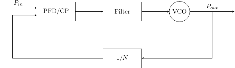 PLL Typical Architecture
Type-I PLL
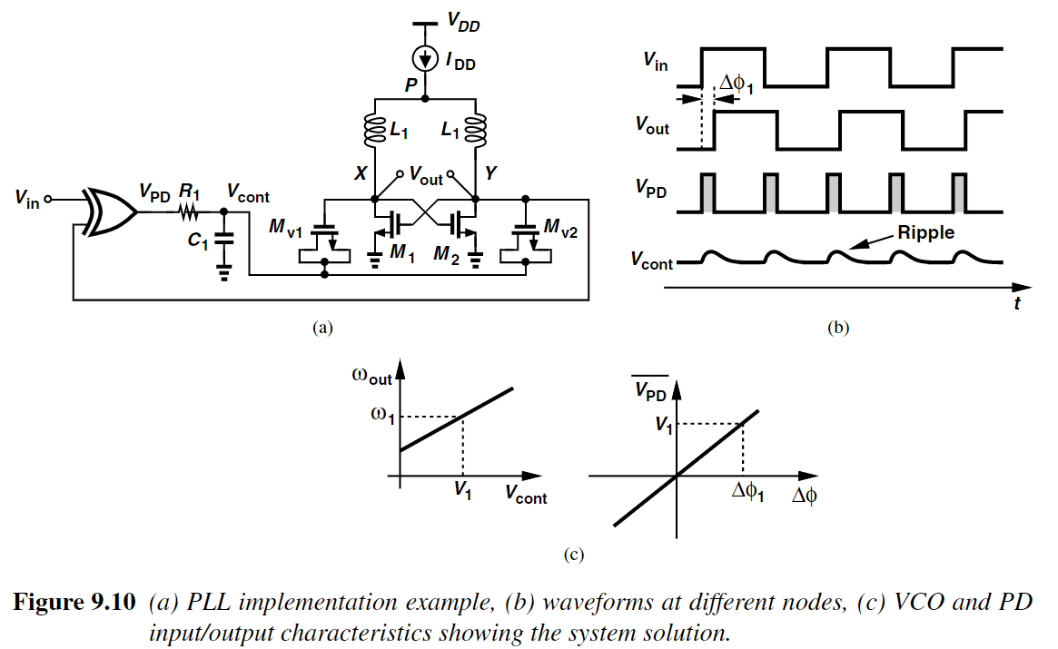
The PLL using XOR as PD is an example of type-I PLL, since there is only one integrator (the VCO) in the loop.
XOR is called PD since phase detectos produce little information if thet sense unequal frequencies at their inputs.
Type-II PLL
The PLL using PFD/CP is an example of type-II PLL, since there are two integrators in the loop.
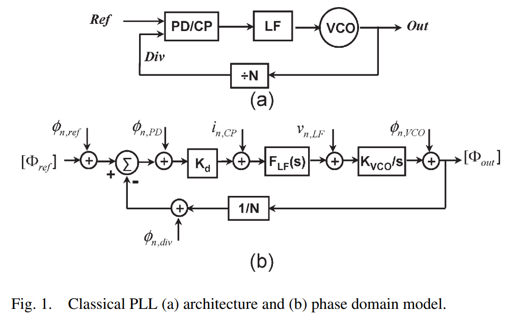
The PLL open-loop transfer function is
\[G(s) = \dfrac{K_d}{N} \cdot F_{LF}(s) \cdot \dfrac{K_{VCO}}{s}\]The VCO phase noise can be expressed by
\[\begin{align} \mathcal{L}_{VCO}(f_m) &= \dfrac{10^{FOM_{VCO}/10}}{P_{VCO}/1mW} \cdot \dfrac{f_{VCO}^2}{f_m^2} \end{align}\]The noise transfer function from VCO to the PLL output is
\[H_{VCO}(s) = \dfrac{1}{1+G(s)}\]Thus the PLL output noise caused VCO can be calculated as
\[\begin{align} \sigma_{t,VCO}^2 &= \dfrac{1}{2\pi^2 f_{out}^2} \cdot \int_{0}^{\infty} \mathcal{L}_{VCO} (f_m) \cdot |H_{VCO}(j2\pi f_m)|^2 df_m \end{align}\]The CP current noise is
\[\begin{align} S_{i,CP} &= 8 kT \gamma g_m \cdot (\tau_{PD}/T_{ref})\\ &= 8kT \gamma \cdot (2 I_{CP}/V_{ov}) \cdot (\tau_{PD}/T_{ref}) \end{align}\]The power of CP is
\[P_{CP} = I_{CP} V_{dd} \cdot (\tau_{PD}/T_{ref}) = I_{CP}V_{dd}\tau_{PD} \cdot f_{ref}\]The in-band phase noise caused by CP is
\[\begin{align} S_{\phi,in-band,CP} &\approx \dfrac{S_{i,CP}}{(K_d/N)^2}\\ &= \dfrac{N^2 f_{ref}^2}{P_{CP}} \cdot \Bigg\{ \tau_{PD}^2 \cdot \dfrac{64\pi^2 kT \gamma V_{dd}}{V_{ov}} \Bigg\} \end{align}\]The output in-band phase noise caused by CP can be expressed by
\[\mathcal{L}_{CP} = \dfrac{1}{2} \cdot S_{\phi,in-band,CP} = \dfrac{10^{FOM_{CP}/10}}{P_{CP}/1mW} \cdot \bigg(\dfrac{f_{out}}{1 Hz}\bigg)^2\]The noise transfer function from CP to the PLL output is
\[H_{CP}(s) = \dfrac{G(s)}{1+G(s)}\]and the PLL output noise caused by CP can be calculated as
\[\sigma_{t,CP}^2 = \dfrac{1}{2\pi^2 f_{out}^2} \cdot \int_{0}^{\infty} \mathcal{L}_{CP} \cdot |H_{CP}(j2\pi f_m)|^2 df_m\]Optimal Bandwidth
use
\[\begin{align} \mathcal{L}_{\mathrm{VCO}} &= \dfrac{\mathcal{L}_{\mathrm{VCO}}(f_r) \cdot f_r^2}{f_m^2}\\ \sigma_{t,\mathrm{VCO}}^2 &= \dfrac{1}{2\pi^2 f_{out}^2} \cdot \int_{0}^{\infty} \mathcal{L}_{\mathrm{VCO}} \cdot \Big| \dfrac{1}{1+G(j2\pi f_m)} \Big|^2 df_m \end{align}\]Assuming a given open-loop transfer function \(G_0(s)\) that results in a closed-loop transfer function with a 3-dB bandwidth of \(f_{c,0}\), scaling the bandwidth to \(f_c\) while keeping the same shape (thus the phase margin) results in a new
\[G(s) = G_{0}(s \cdot \dfrac{f_{c,0}}{f_c})\]then
\[\sigma_{t,\mathrm{VCO}}^2 = \dfrac{2 \mathcal{L}_{\mathrm{VCO}}(f_r)\cdot f_r^2}{f_{out}^2} \cdot \dfrac{f_{c,0}}{f_c} \cdot \int_{0}^{\infty} \Big| \dfrac{1}{s\cdot [1+G_0(s)]} \Big|^2 df\]Also, use
\[\begin{align} \sigma_{t,\mathrm{Loop}}^2 &= \dfrac{1}{2\pi^2 f_{out}^2} \cdot \int_{0}^{\infty} \mathcal{L}_{\mathrm{Loop}} \cdot \Big| \dfrac{G(j2\pi f_m)}{1+G(j2\pi f_m)} \Big|^2 df_m\\ &= \dfrac{\mathcal{L}_{\mathrm{Loop}}}{2\pi^2 f_{out}^2} \cdot \dfrac{f_c}{f_{c,0}} \cdot \int_{0}^{\infty} \Big| \dfrac{G_0(s)}{1+G_0(s)} \Big|^2 df \end{align}\]Thus
\[f_{c,opt} = \sqrt{\dfrac{\mathcal{L}_{\mathrm{VCO}}(f_r)\cdot f_r^2}{\mathcal{L}_{Loop}}} \cdot 2\pi \cdot \sqrt{f_{c,0}^2 \cdot \dfrac{\int_{0}^{\infty}\big|\dfrac{1}{s\cdot[1+G_0(s)]}\big|^2 df}{\int_{0}^{\infty} \big|\dfrac{G_0(s)}{1+G_0(s)}\big|^2 df}}\]then
\[\sigma_{t,\mathrm{PLL,min}}^2 = 2 \sqrt{\dfrac{2 \mathcal{L}_{\mathrm{VCO}}(f_r)\cdot f_r^2}{f_{out}^2} \cdot \dfrac{\mathcal{L}_{\mathrm{Loop}}}{2\pi^2 f_{out}^2} \cdot \int_{0}^{\infty} \big|\dfrac{G_0(s)}{1+G_0(s)}\big|^2 df \cdot \int_{0}^{\infty}\big|\dfrac{1}{s\cdot[1+G_0(s)]}\big|^2 df}\]use
\[\begin{align} \dfrac{\mathcal{L}_{\mathrm{VCO}}(f_r) \cdot f_r^2}{f_{out}^2} &= \dfrac{10^{\mathrm{FOM_{VCO}}/10}}{P_{\mathrm{VCO}}/1 \mathrm{mW}}\\ \dfrac{\mathcal{L}_{\mathrm{Loop}}}{f_{out}^2} &= \dfrac{10^{\mathrm{FOM_{Loop}}/10}}{P_{\mathrm{Loop}}/1 \mathrm{mW}} \end{align}\]then
\[\sigma_{t,\mathrm{PLL,min}}^2 = \dfrac{1}{\sqrt{P_{\mathrm{Loop}}\cdot P_{\mathrm{VCO}}}} \cdot 10^{(\mathrm{FOM_{Loop}+FOM_{VCO}})/20} \cdot \sqrt{\int_{0}^{\infty} \big|\dfrac{G_0(s)}{1+G_0(s)}\big|^2 df \cdot \int_{0}^{\infty}\big|\dfrac{1}{s\cdot[1+G_0(s)]}\big|^2 df} \cdot \dfrac{2}{\pi} \cdot \dfrac{1mW}{1Hz}\]Then with a given power budget, the optimal is \(P_{Loop}=P_{VCO}\)
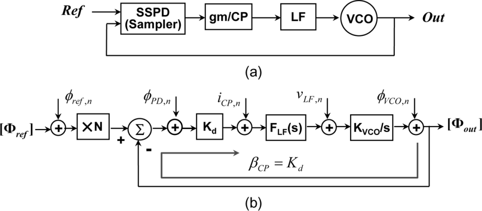
SSPLL