Signal And System Explain

Signal and System

convolution is commutative: proof

from

$$\sum _{k=-\mathrm{\infty }}^{\mathrm{\infty }}x[k]h[n-k]$$

let $k=n-r$

$$\sum _{r=-\mathrm{\infty }}^{\mathrm{\infty }}x[n-r]h[r]$$

LTI system eigen function: proof

$$\begin{array}{rl}y(t)& ={\int }_{-\mathrm{\infty }}^{\mathrm{\infty }}h(\tau )x(t-\tau )d\tau \\ & ={\int }_{-\mathrm{\infty }}^{\mathrm{\infty }}h(\tau )e^{s(t-\tau )}d\tau \\ & =e^{st}{\int }_{-\mathrm{\infty }}^{\mathrm{\infty }}h(\tau )e^{-s\tau }d\tau \end{array}$$ $$\begin{array}{rl}y[n]& =\sum _{k=-\mathrm{\infty }}^{\mathrm{\infty }}h[k]x[n-k]\\ & =\sum _{k=-\mathrm{\infty }}^{\mathrm{\infty }}h[k]z^{n-k}\\ & =z^n\sum _{k=-\mathrm{\infty }}^{\mathrm{\infty }}h[k]z^{-k}\end{array}$$

Paeseval’s theorem: proof

$$\begin{array}{rl}& \sum _{k=-\mathrm{\infty }}^{\mathrm{\infty }}|a_k{|}^2\\ =& \sum _{k=-\mathrm{\infty }}^{\mathrm{\infty }}{a}_k{a}_k^{\ast }\\ =& \sum _{k=-\mathrm{\infty }}^{\mathrm{\infty }}{a}_k{\displaystyle \frac{1}{T}}{\int }_T{x}^{\ast }(t)e^{jk{\omega }_{0}t}dt\\ =& {\displaystyle \frac{1}{T}}\sum _{k=-\mathrm{\infty }}^{\mathrm{\infty }}{\int }_T{x}^{\ast }(t)a_k{e}^{jk{\omega }_{0}t}dt\\ =& {\displaystyle \frac{1}{T}}{\int }_T{x}^{\ast }(t)\sum _{k=-\mathrm{\infty }}^{\mathrm{\infty }}{a}_k{e}^{jk{\omega }_{0}t}dt\\ =& {\displaystyle \frac{1}{T}}{\int }_T{x}^{\ast }(t)x(t)dt\end{array}$$ $$\begin{array}{rl}& \sum _{k=0}^{N-1}|a_k{|}^2\\ =& \sum _{k=0}^{N-1}{a}_k{a}_k^{\ast }\\ =& \sum _{k=0}^{N-1}{a}_k{\displaystyle \frac{1}{N}}\sum _{n=0}^{N-1}{x}^{\ast }[n]e^{jk{\omega }_{0}n}\\ =& {\displaystyle \frac{1}{N}}\sum _{n=0}^{N-1}{x}^{\ast }[n]\sum _{k=0}^{N-1}{a}_k{e}^{jk{\omega }_{0}n}\\ =& {\displaystyle \frac{1}{N}}\sum _{n=0}^{N-1}{x}^{\ast }[n]x[n]\end{array}$$

Fourier Transform

Fourier Transform: proof

$$\begin{array}{rl}x(t)& =\sum _{k=-\mathrm{\infty }}^{\mathrm{\infty }}({\int }_{T}x(\tau )e^{-jk{\omega }_0\tau }d\tau )e^{jk{\omega }_{0}t}{\displaystyle \frac{1}{T}}\\ & ={\displaystyle \frac{1}{2\pi }}\sum _{k=-\mathrm{\infty }}^{\mathrm{\infty }}({\int }_{T}x(\tau )e^{-jk{\omega }_0\tau }d\tau )e^{jk{\omega }_{0}t}{\displaystyle \frac{2\pi }{T}}\\ & ={\displaystyle \frac{1}{2\pi }}\sum _{k=-\mathrm{\infty }}^{\mathrm{\infty }}({\int }_{T}x(\tau )e^{-jk{\omega }_0\tau }d\tau )e^{jk{\omega }_{0}t}{\omega }_0\\ & ={\displaystyle \frac{1}{2\pi }}{\int }_{-\mathrm{\infty }}^{\mathrm{\infty }}X(j\omega )e^{j\omega t}d\omega \end{array}$$ $$X(j\omega )={\int }_{-\mathrm{\infty }}^{\mathrm{\infty }}x(t)e^{-j\omega t}dt$$

book_xinhaoyuxianxingxitongfenxi

Intro

Signal

Continuous-Time Signal and Discrete-Time Signal

Periodic Signal and Non-Periodic Signal

Real Signal and Complex Signal

• Deterministic signal, stochastic signal.
• Continuous-time signal, discrete-time signal.
• Periodic signal, non-periodic signal.
• Energy signal, power signal.
• Causal signal, anti-causal signal.

The total energy and average power of a signal $f(t)$ is

$$\begin{array}{rl}E& ={\int }_{-\mathrm{\infty }}^{\mathrm{\infty }}|f(t){|}^{2}dt\\ P& =\underset{T\to \mathrm{\infty }}{lim}{\displaystyle \frac{1}{T}}{\int }_{-T/2}^{T/2}|f(t){|}^{2}dt\end{array}$$

• Energy signal: $E<\mathrm{\infty }$. Clearly it implies $P=0$.
• Power signal: $0<P<\mathrm{\infty }$. Clearly it implies $E=\mathrm{\infty }$.
• Causal signal: $f(t)=0\mathrm{\forall }t<0$.
• Anti-causal signal: $f(t)=0\mathrm{\forall }t\ge 0$.

Step function

$$u(t)=\{\begin{array}{ll}0,& t<0\\ 1,& t>0\end{array}$$

the value at $t=0$ is not important, as long as we define $u(0)<\mathrm{\infty }$. Since in the theory of generalized function, it is always evaluated by integration.

Impulse function is defined by using generalized function. For well behaved function $\varphi (t)$, impulse function $\delta (t)$ is the function that satisfy

$${\int }_{-\mathrm{\infty }}^{\mathrm{\infty }}\delta (t)\varphi (t)dt=\varphi (0)$$

e.g.,

$$\begin{array}{rl}\delta (t)& =\underset{b\to \mathrm{\infty }}{lim}b{e}^{-\pi (bt{)}^2}\\ \delta (t)& =\underset{b\to \mathrm{\infty }}{lim}{\displaystyle \frac{\sin (bt)}{\pi t}}\end{array}$$

• The derivitive of $\delta (t)$

using $f(t){\delta }^{\prime }(t)=f(0){\delta }^{\prime }(t)-f^{\prime }(0)\delta (t)$, we have

$${\int }_{-\mathrm{\infty }}^{\mathrm{\infty }}f(t){\delta }^{\prime }(t)dt=-f^{\prime }(0)$$

and also

$${\int }_{-\mathrm{\infty }}^{\mathrm{\infty }}f(t){\delta }^{(n)}(t)dt=(-1{)}^n{f}^{(n)}(0)$$

another equation (can only be used in the integral)

$$\begin{array}{rl}\delta (at)& ={\displaystyle \frac{1}{|a|}}\delta (t)\\ {\delta }^{(n)}(at)& ={\displaystyle \frac{1}{|a|}}{\displaystyle \frac{1}{a^n}}{\delta }^{(n)}(t)\end{array}$$

• In summary
  • The definitions
    •   ${\int }_{-\mathrm{\infty }}^{\mathrm{\infty }}f(t){\delta }^{(n)}(t)dt=(-1{)}^n{f}^{(n)}(0)$
  • The formula can be used in anywhere (e.g., in the arguments for the derivitive definition)
    •   $f(t){\delta }^{(n)}(t)=f(0){\delta }^{(n)}(t)$
  • The formula can only be used in the integral
    •   ${\delta }^{(n)}(at)={\displaystyle \frac{1}{|a|}}{\displaystyle \frac{1}{a^n}}{\delta }^{(n)}(t)$
    •   $f(t){\delta }^{\prime }(t)=f(0){\delta }^{\prime }(t)-f^{\prime }(0)\delta (t)$
• Exercises

$$\begin{array}{rl}{\int }_{-\mathrm{\infty }}^{\mathrm{\infty }}{\displaystyle \frac{\sin (2t)}{t}}\delta (t)dt& =\underset{t\to 0}{lim}{\displaystyle \frac{\sin (2t)}{t}}=2\end{array}$$ $$\begin{array}{rl}{\int }_{-\mathrm{\infty }}^{\mathrm{\infty }}(t^3-3t^2+5t-1){\delta }^{\prime }(t-1)dt& =-g^{\prime }(1)=-2\end{array}$$ $${\int }_{-\mathrm{\infty }}^{\mathrm{\infty }}(t^3+5)\delta ({\displaystyle \frac{t}{2}})dt=2{\int }_{-\mathrm{\infty }}^{\mathrm{\infty }}(t^3+5)\delta (t)dt=10$$ $$\begin{array}{r}{\int }_{-\mathrm{\infty }}^t(2-x){\delta }^{\prime }(x)dx={\int }_{-\mathrm{\infty }}^t[2{\delta }^{\prime }(x)-(-1)\delta (t)]dt=2\delta (t)+u(t)\end{array}$$

• Discrete-time impulse and step function

$$u[k]=\{\begin{array}{l}1,k\ge 0\\ 0,k<0\end{array}$$ $$\sum _{k=-\mathrm{\infty }}^{\mathrm{\infty }}f[k]\delta [k]=f[0]$$

Discrete-time difference

$$\delta [k]=u[k]-u[k-1]$$

Discrete-time summation

$$u[k]=\sum _{i=-\mathrm{\infty }}^k\delta [i]$$

Decomposition

$$u[k]=\sum _{j=0}^{\mathrm{\infty }}\delta [k-j]$$

• Signal reflect, move, and scale
  • give the waveform $f(t)$, $f(-t)$ is reflect at 0. $(t\times -1)$
  • give the waveform $f(t+2)$, $f(-t+2)$ is reflect at 0. $(t\times -1)$
  • give the waveform $f(t)$, $f(t-3)$ is move right to 3 units. $(t-3)$
  • give the waveform $f(t+2)$, $f(t-1)$ is move right to 3 units. $(t-3)$
  • give the waveform $f(t)$, $f(3t)$ is shrink 3 times at 0. $(t\times 3)$
  • give the waveform $f(t+2)$, $f(3t+2)$ is shrink 3 times at 0. $(t\times 3)$
  • give the waveform $f(t)$, $f(0.2t)$ is expand 5 times at 0. $(t\times 0.2)$
  • give the waveform $f(t+3)$, $f(0.2t+3)$ is expand 5 times at 0. $(t\times 0.2)$

• Usually first move, then scale, then reflect.

• Do derivitive one the waveform, add the impulse function.

Introduction to System

• Linear system

$$T[a{f}_1(.)+b{f}_2(.)]=aT[f_1(.)]+bT[f_2(.)]$$

• Dynamic linear system
  •   $y(t)=y_{zi}(t)+y_{zs}(t)$
  • The system are linear for the input and states respectively.

$$y(.)=y_{zs}(.)+y_{zi}(.)$$ $$T[\{a{f}_1(t)+b{f}_2(t)\},\{0\}]=aT[\{f_1(.)\},\{0\}]+bT[\{f_2(.)\},\{0\}]$$ $$T[\{0\},\{a{x}_1(0)+b{x}_2(0)\}]=aT[\{0\},\{x_1(0)\}]+bT[\{0\},\{x_2(0)\}]$$

• Time varying or time invariant: only look zero state response.

$$T[\{0\},f(t-td)]=y_{zs}(t-t_d)$$

• LTI system.
  • if $f(t)\to y_{zs}(t)$, then $f^{\prime }(t)\to y_{zs}^{\prime }(t)$
  • if $f(t)\to y_{zs}(t)$, then ${\int }_{-\mathrm{\infty }}^{t}f(x)dx\to {\int }_{-\mathrm{\infty }}^t{y}_{zs}(x)dx$
  • TODO: how to prove?
• Causal system and non-causal system.
  • It is defined for $y_{zs}(t)$
• Example:

For a causal LTI causal system with initial state $x(0\mathrm{\_})$, if $x(0\mathrm{\_})=1$ and with a causal input $f_1(t)$, the full response is

$$y_1(t)=[e^{-t}+\cos (\pi t)]u(t)$$

if $x(0\mathrm{\_})=2$ and input $3f_1(t)$, the full response is

$$y_2(t)=[-2e^{-t}+3\cos (\pi t)]u(t)$$

then for input $f_1^{\prime }(t)+2f_1(t-1)$, find the zero state response.

• Solution: $y_{zs}(t)=-3\delta (t)+[4e^{-t}-\pi \sin (\pi t)]u(t)+2\{-4e^{-(t-1)}+\cos [\pi (t-1)]\}u(t-1)$

Continuous-Time Time-Domain Analysis

Response of LTI System

Differential Equations

The differential equation

$$a_2{\displaystyle \frac{d^{2}y(t)}{d{t}^2}}+a_1{\displaystyle \frac{y(t)}{dt}}+a_{0}y(t)=f(t)$$

with initial conditions $y(0_{+}),y^{\prime }(0_{+})$

we can determine the responses for the given $f(t)$ and initial conditions.

Block Diagram of Differential Equations

Take the example of

$$y^{″}(t)+a{y}^{\prime }(t)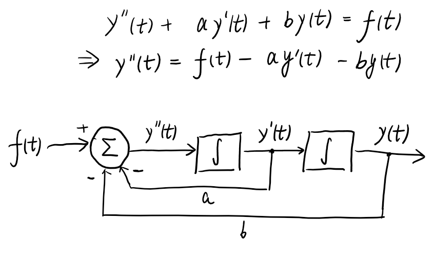+by(t)=f(t)$$

Another example

$$y^{″}(t)+3y^{\prime }(t)+2y(t)=4f^{\prime }(t)+f(t)$$

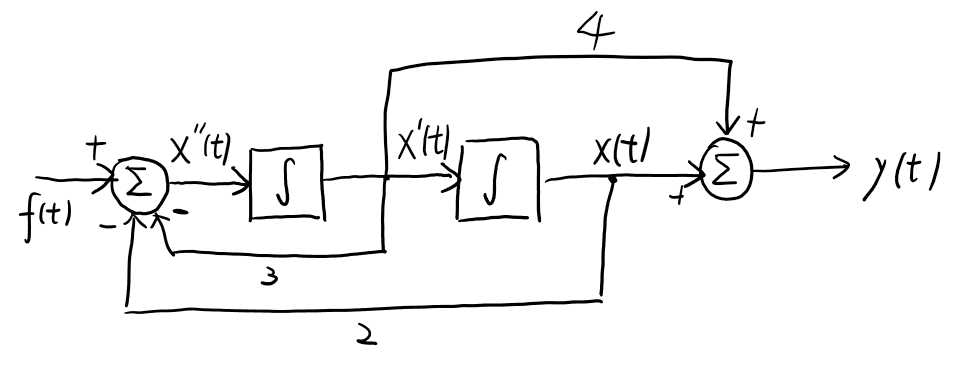
Classic Solution of Differential Equations

If $f(t)$ has finite derivative up to $f^{(m)}(t)$, for differential equations

$$\begin{array}{rl}& y^{(n)}(t)+a_{n-1}{y}^{(n-1)}(t)+\cdots +a_1{y}^{(1)}(t)+a_{0}y(t)\\ & =b_m{f}^{(m)}(t)+b_{m-1}{f}^{(m-1)}(t)+\cdots +b_1{f}^{(1)}(t)+b_{0}f(t)\end{array}$$

and $n$ initial conditions

$$y^{(n-1)}(0),y^{(n-2)}(0),\dots ,y(0)$$

The solution is composed of homogeneous solution and special solution

$$y(t)=y_h(t)+y_p(t)$$

where homogeneous solution is the complete solution of the homogeneous differential equation with all possible initial conditions

$$y^{(n)}(t)+a_{n-1}{y}^{(n-1)}(t)+\cdots +a_1{y}^{(1)}(t)+a_{0}y(t)=0$$

the corresponding eigen-function has $n$ roots

$$F(\lambda )={\lambda }^n+a_{n-1}{\lambda }^{n-1}+\cdots +a_1\lambda +a_0=0$$

If the $n$ roots ${\lambda }_1,\dots ,{\lambda }_n$ are not equal to each other

$$y_h(t)=C_1{e}^{{\lambda }_{1}t}+C_2{e}^{{\lambda }_{2}t}+\cdots +C_n{e}^{{\lambda }_{n}t}$$

If there are $e_i$ same roots $\lambda$, the corresponding term is

$$(C_0+C_{1}t+\cdots +C_{e_i-1}{t}^{e_i-1})e^{\lambda t}$$

and the special solution is one arbitrary solution satisfy the original differential equation without worring about the initial condition.

TODO: finish the table for special solution.

Example:

$$\begin{array}{rl}& y^{″}(t)+5y^{\prime }(t)+6y(t)=f(t)\\ & f(t)=2e^{-t},t\ge 0\\ & y^{\prime }(0)=-1,y(0)=2\end{array}$$

On Initial Conditions

Zero Input Response

Zero State Response

Deprecated

Discrete-Time Signals

The definition of discrete-time signal is a function from non-negative integer set to real number set.

$$f:{\mathbb{Z}}_{\ge 0}\to R$$

Basic Signals

• the discrete-time impulse function

$$\delta [k]=\{\begin{array}{ll}1,& k=0\\ 0,& k>0\end{array}$$

• the discrete-time unit step function

$$u[k]=1$$

• the discrete-time ramp signal

$$r[k]=k$$

The $z$-transform

Instead of describing the value at each point, there is another way to describe a signal by only using one single equation, that is $Z$-transform.

$$F(z)=\sum _{k=0}^{\mathrm{\infty }}f[k]z^{-k}$$

It can be proved its ROC is

$$|z|>r_1=\underset{k\to \mathrm{\infty }}{lim sup}|f[k]{|}^{1/k}$$

Please note the term ROC doesn’t literally match to “region of convergence”, since we always neglect $r_1$, whether $F(z)$ really converge at $r_1$ or not.

Signal $x[.]{\mathbb{Z}}_{\ge 0}\to \mathrm{R}$	$z$-Transform	ROC	Notes
$\delta [.]$	$1$	$|z|>0$
$u[n]=1$	${\displaystyle \frac{1}{1-z^{-1}}}$	$|z|>1$
$r[n]=n$	${\displaystyle \frac{z^{-1}}{(1-z^{-1}{)}^2}}$	$|z|>1$
$x[n]=a^n$	${\displaystyle \frac{z}{z-a}}$	$|z|>|a|$
$x[n]=f[n]+g[n]$	$F(z)+G(z)$	$\mathrm{ROC}\supseteq \mathrm{ROC}(f)\cap \mathrm{ROC}(g)$	$\mathrm{ROC}(f)\cap \mathrm{ROC}(g)\ne \mathrm{\varnothing }$
$x[n]=af[n],a\ne 0$	$aF(z)$	$\mathrm{ROC}=\mathrm{ROC}(f)$	$\mathrm{ROC}(f)\ne \mathrm{\varnothing }$
$x[n]=f_{delay,m}[n]$	$z^{-m}F(z)$	$\mathrm{ROC}=\mathrm{ROC}(f)$	$\mathrm{ROC}(f)\ne \mathrm{\varnothing }$
$x[n]=(f\ast g)[n]$	$F(z)G(z)$	$\mathrm{ROC}\supseteq \mathrm{ROC}(f)\cap \mathrm{ROC}(g)$	$\mathrm{ROC}(f)\cap \mathrm{ROC}(g)\ne \mathrm{\varnothing }$
$x[n]=f[n]-f_{delay,1}[n]$	$(1-z^{-1})F(z)$	$\mathrm{ROC}\supseteq \mathrm{ROC}(f)$	Difference

• Almost all the discrete-time signals in practice will have $z$-Transform with some $\mathrm{ROC}\ne \mathrm{\varnothing }$. Although signals like $x[n]=n^n$ doesn’t have $z$-Transform, perhaps they never appear in real practice.

• Time delayed by $m$ with initial rest is defined as

$$f_{delay,m}[n]=\{\begin{array}{ll}0,& n<m\\ f[n-m],& n\ge m\end{array}$$

• Convolution is defined as

$$(f\ast g)[n]=\sum _{k=0}^{n}f[k]g[n-k]=\sum _{k=0}^{n}f[n-k]g[k]$$

below is how to visualize the convolution for $F(z)=1+z^{-1}+z^{-2}$ and $G(z)=1+z^{-1}+z^{-2}+z^{-3}$.

From Time-Domain to $z$-Domain

From $z$-Domain to Time-Domain

Discrete-Time Systems

$$y[.]=a_{0}x[.]+a_1\cdot x_{delay,1}[.]+a_2\cdot x_{delay,2}[.]+\cdots +a_m\cdot x_{delay,m}[.]+b_1\cdot y_{delay,1}[.]+b_2\cdot y_{delay,2}[.]+\cdots +b_r\cdot y_{delay,r}[.]$$

Example 01

$$x[k]=\{\begin{array}{ll}1,& k=0,1,2\\ 0,& \text{otherwise}\end{array}$$ $$X(z)=1+z^{-1}+z^{-2},\mathrm{ROC}=\{z\ne 0\}$$

Example 02

$$x[k]=a^n+1$$ $$X(z)={\displaystyle \frac{1}{1-z^{-1}}}+{\displaystyle \frac{z}{z-a}},\mathrm{ROC}=\{|z|>\max (1,|a|)\}$$

Example 03

$$\begin{array}{rl}{u}_{delay,1}[n]& =\{\begin{array}{ll}0,& k=0\\ 1,& k>0\end{array}\\ U_{delay,1}(z)& ={\displaystyle \frac{z^{-1}}{1-z^{-1}}},\mathrm{ROC}=\{|z|>1\}\end{array}$$

Example 04

calculate the difference of $u[.]$

$$\begin{array}{rl}u[.]-u_{delay,1}[.]& =\delta [.]\\ (1-z^{-1})\cdot {\displaystyle \frac{1}{1-z^{-1}}}& =1,\mathrm{ROC}=\{|z|>0\}\end{array}$$

Theorem 01

Let $f[.]$ and $g[.]$ be discrete-time signals with

$$\mathrm{ROC}(f)\cap \mathrm{ROC}(g)\ne \mathrm{\varnothing }$$

If $F(z)=G(z)$ for $z\in \mathrm{ROC}(f)\cap \mathrm{ROC}(g)$, then $f[k]=g[k]$ for all $k\in \mathbb{Z}$

• It implies, for an unkown signal $f[.]$, if we know its $F(z)$ expression and its $\mathrm{ROC}(f)$ is non empty, then in principle we completely know the signal.
• So, we have a two directional table!

Example 05

Calculate the $z$-Transform of $x[n]=n+1$, without calculate explicitly.

We know $x[.]$ must have $X(z)$ in $\mathrm{ROC}(x)\ne \mathrm{\varnothing }$. $\leftarrow$ ROC $lim sup$ rule.

$x_{delay,1}[.]$ have $z$-Transform $z^{-1}X(z)$ in $\mathrm{ROC}(x)$. $\leftarrow$ $z$-Transform of time delay.

$x_{delay,1}[.]=r[.]$, which has $z$-Transform ${\displaystyle \frac{z^{-1}}{(1-z^{-1}{)}^2}}$ with $\mathrm{ROC}=\{|z|>1\}$. $\leftarrow$ table

So, $X(z)={\displaystyle \frac{1}{(1-z^{-1}{)}^2}}$ with $\mathrm{ROC}(x)=\{|z|>1\}$.

Example 06

Calculate the signal $(u\ast u)[.]$.

Let $g[.]=(u\ast u)[.]$, then $G(z)={\displaystyle \frac{1}{(1-z^{-1}{)}^2}}$ for $\mathrm{ROC}(g)\supseteq \{|z|>1\}$ $\leftarrow$ convolution.

Then $(u\ast u)[n]=g[n]=n+1\leftarrow$ table

Example 07 (Summation)

define $x_{sum}[.]$ with

$$x_{sum}[n]=\sum _{k=0}^{n}x[k]$$

Then if exists $X(z)$ with $\mathrm{ROC}(x)\ne \mathrm{\varnothing }$ and $X_{sum}(z)$ with $\mathrm{ROC}(x_{sum})\ne \mathrm{\varnothing }$, then

$$\begin{array}{rl}{X}_{sum}(z)& ={\displaystyle \frac{X(z)}{1-z^{-1}}}\text{ with }\mathrm{ROC}(x_{sum})\\ \mathrm{ROC}(x_{sum})& \subseteq \mathrm{ROC}(x)\end{array}$$

LUT Exercises

TODO

NOT

Discrete-Time LTI Systems

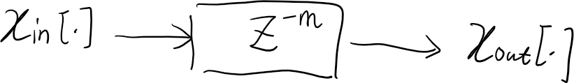
A system will transform a input signal $x_{in}[.]$ to an output signal $x_{out}[.]$

$$x_{out}[.]=H(z)\{x_{in}[.]\}$$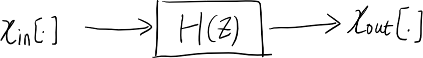

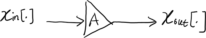
Basic Systems and Block Diagram

• Amplify or attennuation or identity.

$$x_{out}[.]=A\cdot x_{in}[.]$$

• Delayed by $m$

$$x_{out}[.]=x_{in}[.-m]$$

• Superposition

$$x_{out}[.]=H_1(x)\{x_{in}[.]\}+H_2(x)\{x_{in}[.]\}$$

• Cascade

• Feedback

link

Discrete-Time Systems

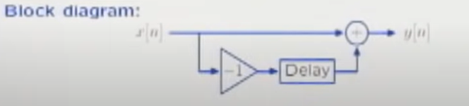
$y[n]=x[n]-x[n-1]$ is an example of difference equation.

this drawing explains how to reflect $x[n-1]$ is delayed $x[x]$.

Knowing that $x[n-1]$ is the delayed $x[n]$, the difference equation can also be represented by a block diagram.

Let $x[n]$ equal the “unit sample” signal $\delta [n]$ (the most simple non-trivial signal you can imagine!)

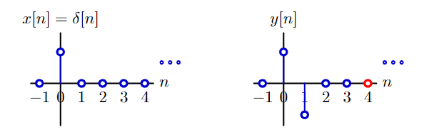
To be more precise, we need to mention the systen start “at rest”, meaning all the output at the delay start at 0. Then you can completely compute the output $y[n]$ for any input $x[n]$, without any ambigious.

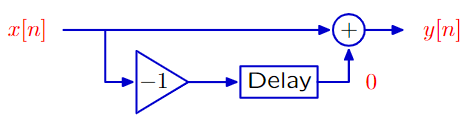
Is there any differences between the difference equation and block diagram?

• operators in the block diagram are more easier to be understood as an manipulation of the whole signal, instead of just single samples.

We can denote the delay operator as $z^{-1}$. This drawing shows how the $z^{-1}$ signal is applied to the unit sample signal. The the block diagram can be denoted by

$$1-z^{-1}$$