Spectral Analysis
Let’s review spectral analysis of deterministic signal.
If \(x(t)\) is periodic signal with period \(T\), we have Fourier series.
\[x(t) = \sum_{k=-\infty}^{\infty} \alpha_k e^{j \omega_k t}\]where
\[\omega_k = \dfrac{2k\pi}{T}\]and
\[\alpha_{k} = \dfrac{1}{T} \int_{-\frac{T}{2}}^{\frac{T}{2}} x(t) e^{-j \omega_k t} dt\]It can be written as
\[\begin{align} x(t) &= \dfrac{1}{T} \sum_{k=-\infty}^{\infty} \bigg( \int_{-\frac{T}{2}}^{\frac{T}{2}} x(s) \exp(-j \dfrac{2 k \pi}{T} s) ds \bigg) \exp(j \dfrac{2k \pi}{T} t) \end{align}\]Integral is the limit of summation in the sense of
\[\int f(x)dx = \sum_{k} f(x_k) (x_k - x_{k-1}) = \sum_{k} f(x_k) \Delta x_k, \quad \text{ when } \Delta x_k \to 0\]thus
\[\begin{align} x(t) &= \dfrac{1}{2\pi} \sum_{k=-\infty}^{\infty} \bigg( \int_{-\frac{T}{2}}^{\frac{T}{2}} x(s) \exp(-j \dfrac{2 k \pi}{T} s) ds \bigg) \exp(j \dfrac{2k \pi}{T} t) \cdot \dfrac{2\pi }{T}\\ &= \dfrac{1}{2\pi} \int_{-\infty}^{\infty} \hat{X}(\omega) \exp(j \omega t) d\omega \end{align}\]where
\[\hat{X}(\omega) = \int_{-\infty}^{\infty} x(t) \exp(-j \omega t) dt\]and the fourier transfer exists if \(x(t)\) is absolute integrable.
\[\int_{-\infty}^{\infty} \vert x(t) \vert dt < \infty\]this is one fundamental difficulty for stationary random process.
Power Spectral Density
For a W.S.S. \(X(t)\), we can try to do this
\[\begin{align} &\dfrac{1}{T} E \bigg\vert \int_{-\frac{T}{2}}^{\frac{T}{2}} X(t) \exp(-j \omega t) dt \bigg\vert^2\\ =& \dfrac{1}{T} E \bigg(\int_{-\frac{T}{2}}^{\frac{T}{2}} X(t) \exp(-j\omega t) dt \bigg) \cdot \bigg( \int_{-\frac{T}{2}}^{\frac{T}{2}} \overline{X(s)} \exp(j \omega s) ds \bigg)\\ =& \dfrac{1}{T} \int_{-\frac{T}{2}}^{\frac{T}{2}} \int_{-\frac{T}{2}}^{\frac{T}{2}} E(X(t)\overline{X(s)}) \exp(-j\omega (t-s)) \mathrm{d}t \mathrm{d}s\\ = & \dfrac{1}{T} \int_{-\frac{T}{2}}^{\frac{T}{2}} \int_{-\frac{T}{2}}^{\frac{T}{2}} R(t-s) \exp(-j\omega (t-s)) \mathrm{d}t \mathrm{d}s \end{align}\]substitude variable, \(u=t-s, \quad v = t+s\), we need to take variable carefully in the range, the function, and the absolute value of the Jacobian determinant.
\[\begin{align} \mathrm{d}t\mathrm{d}s = \bigg\vert \mathrm{det} \dfrac{\partial(t,s)}{\partial (u,v)} \bigg\vert \mathrm{d}u \mathrm{d} v \end{align}\]remember that for square matrix \(A, B\), \(\vert A B \vert = \vert A \vert \cdot \vert B \vert\), and \(\bigg( \dfrac{\partial(t,s)}{\partial(u,v)} \bigg)^{-1} = \dfrac{\partial (u,v)}{\partial (t,s)}\)
thus \(\mathrm{d} t \mathrm{d} s = \bigg\vert \dfrac{\partial (u,v)}{\partial (t,s)} \bigg\vert^{-1} \mathrm{d} u \mathrm{d}v\)
and
\[\dfrac{\partial (u,v)}{\partial (t,s)} = \begin{bmatrix} \dfrac{\partial u}{\partial t} & \dfrac{\partial u}{\partial s}\\ \dfrac{\partial v}{\partial t} & \dfrac{\partial v}{\partial s} \end{bmatrix} = \begin{bmatrix} 1 & -1\\ 1 & 1 \end{bmatrix}\]thus
\[\mathrm{d} t \mathrm{d} s = \bigg\vert \dfrac{\partial (u,v)}{\partial (t,s)} \bigg\vert^{-1} \mathrm{d} u \mathrm{d}v = \dfrac{1}{2} \mathrm{d} u \mathrm{d} v\]to deal with the range, we need to draw the diagram. As long as the original range is the conventional direction, we can use the conventional direction for the new integral
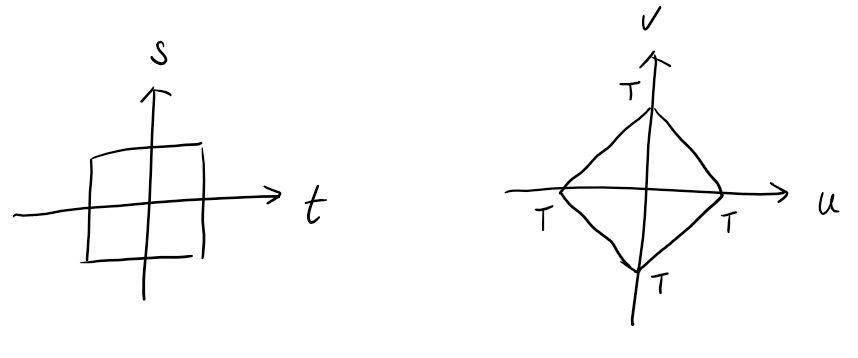
thus
\[\begin{align} &\dfrac{1}{2T} \bigg( \int_{-T}^{0} \int_{-T-u}^{T+u} + \int_{0}^{T} \int_{-T+u}^{T-u} \bigg) R(u)\exp(-j\omega u) \mathrm{d} v \mathrm{d} u\\ =&\dfrac{1}{2T} \int_{-T}^{T} \int_{-T+\vert u \vert}^{T- \vert u\vert} R(u)\exp(-j\omega u) \mathrm{d} v \mathrm{d} u\\ =&\dfrac{1}{2T} \int_{-T}^{T} (2T - 2 \vert u \vert) R(u)\exp(-j\omega u) \mathrm{d} u\\ =& \int_{-T}^{T} \Big(1 - \dfrac{ \vert u \vert}{T}\Big) R(u)\exp(-j\omega u) \mathrm{d} u \end{align}\]let \(T \to \infty\)
\[\dfrac{1}{T} E \bigg\vert \int_{-\frac{T}{2}}^{\frac{T}{2}} X(t) \exp(-j \omega t) dt \bigg\vert^2 = \int_{-\infty}^{\infty} R(u) \exp(-j\omega u) du = S(\omega)\]This is called Wiener-Khinchine theorem. It is interesting to note here, if assume \(R(u)\) is real function, since \(R(u)\) is positive definite function (thus it is also symmetry), we know its Fourier transfer is real and symmetry, and positive for all \(\omega\), meets the idea of power spectral density. Thus
\[\begin{align} S(\omega) &= \int_{-\infty}^{\infty} R(t) \cos(\omega t) dt\\ R(t) &= \dfrac{1}{2\pi} \int_{-\infty}^{\infty} S(\omega) \cos(\omega t) d\omega \end{align}\]LTI Responses
Assumes a W.S.S. process \(X(t)\) with PSD \(S(\omega)\) passing through a LTI system with impulse response \(h(t)\), we know
\[Y(t) = \int_{-\infty}^{\infty} h(t-\tau) X(\tau) d\tau\]then
\[\begin{align} &R_{Y}(t,s) = E(Y(t) \overline{Y(s)}) = E \bigg(\int_{-\infty}^{\infty} h(t-\tau) X(\tau) d\tau \bigg) \overline{\bigg(\int_{-\infty}^{\infty} h(s-r)X(r)dr\bigg)}\\ =& \int_{-\infty}^{\infty} \int_{-\infty}^{\infty} R_{X}(\tau-r) h(t-\tau) \overline{h(s-r)} d\tau dr \end{align}\]to see if the integral is a convolutoin, the summation of all the variable in the function, has to cancel all the integral variable, and it gives the convolutoin at the value of the summation.
We need to define
\[\tilde{h}(t) = \overline{h(-t)}\]then
\[\begin{align} R_{Y}(t,s) &= \int_{-\infty}^{\infty} \int_{-\infty}^{\infty} R_{X}(\tau-r) h(t-\tau) \overline{h(s-r)} d\tau dr\\ &= \int_{-\infty}^{\infty} \int_{-\infty}^{\infty} R_{X}(\tau-r) h(t-\tau) \tilde{h}(r-s) d\tau dr\\ &= R_{X} * h * \tilde{h} (t-s) \end{align}\]thus it is clear \(Y(t)\) is W.S.S., also
\[S_Y(\omega) = S_X(\omega)\cdot H(\omega) \cdot \tilde{H}(\omega)\]and
\[\begin{align} \tilde{H}(\omega) &= \int_{-\infty}^{\infty} \tilde{h}(t) \exp(-j\omega t) dt\\ &= \int_{-\infty}^{\infty} \overline{h(-t)} \exp(-j\omega t) dt\\ &= \overline{\int_{-\infty}^{\infty} h(-t) \exp(j\omega t) dt}\\ &= \overline{\int_{-\infty}^{\infty} h(\tau) \exp(-j\omega \tau) d\tau}\\ &= \overline{H(\omega)} \end{align}\]thus
\[S_Y(\omega) = S_X(\omega) \cdot H(\omega) \cdot \overline{H(\omega)} = S_X(\omega) \vert H(\omega) \vert^2\]Common PSDs And Their Autocorrelations
Please note that the Fourier transform is not the same (or similar) as Laplace transform table, since the table we usually see is for single sided functions.
\[\begin{align} S(\omega) &= \int_{-\infty}^{\infty} R(\tau) \exp(-j\omega\tau)d\tau\\ R(\tau) &= \dfrac{1}{2\pi}\int_{-\infty}^{\infty} S(\omega) \exp(j\omega\tau) d\omega \end{align}\]or using frequency (Hz) instead of angular frequency
\[\begin{align} S(f) &= \int_{-\infty}^{\infty}R(\tau)\exp(-j2\pi f \tau) d\tau\\ R(\tau) &= \int_{-\infty}^{\infty} S(f) \exp(j2\pi f \tau) df \end{align}\]White Noise
For a white noise with two-sided PSD
\[S(f) = N_0\]The autocorrelation is
\[R(\tau) = N_0 \delta(\tau)\]We can verify it by
\[\int_{-\infty}^{\infty} N_0 \delta(\tau) \exp(-j2\pi f\tau) d\tau = N_0\]Note that the directly apply of the inverse Fourier transform may seems difficult.
Lowpass Noise
For a two-sided PSD
\[S(f) = \dfrac{N_0}{1+\big(\dfrac{f}{f_b}\big)^2}\]or
\[S(\omega) = \dfrac{N_0 \cdot \omega_b^2}{\omega_b^2+\omega^2}\]using the formula
\[\int_{-\infty}^{\infty} \dfrac{1}{a^2+\omega^2} \cdot \exp(j\omega t)d \omega = \dfrac{\pi}{a} \cdot \exp(-a\vert t \vert), \quad a > 0\] \[\begin{align} R(\tau) &= \dfrac{1}{2\pi} \int_{-\infty}^{\infty} \dfrac{N_0 \cdot \omega_b^2}{\omega_b^2 + \omega^2} \cdot \exp(j\omega \tau) d\omega\\ &= \dfrac{1}{2\pi} \cdot N_0 \cdot \omega_b^2 \cdot \dfrac{\pi}{\omega_b} \cdot \exp(-\omega_b \vert \tau \vert)\\ &= \pi f_b \cdot N_0 \cdot \exp(-2\pi f_b \vert \tau \vert) \end{align}\]We can do a quick sanity check, since the effective power bandwidth is \(\pi f_b/2\), we should have
\[2N_0 \cdot \dfrac{\pi}{2} \cdot f_b = \pi f_b \cdot N_0\]LTV Responses
Without the assumption of W.S.S. process, we need to derive the PSD again by
\[\begin{align} & \dfrac{1}{T} E \left\vert \int_{-T/2}^{T/2} X(t)\exp(-j\omega t) dt \right\vert^2\\ = & \dfrac{1}{T} E\left(\int_{-T/2}^{T/2} X(t)\exp(-j\omega t) dt\right) \left( \int_{-T/2}^{T/2} \overline{X(s)}\exp(j\omega s)\right)\\ = & \dfrac{1}{T} \int_{-T/2}^{T/2} \int_{-T/2}^{T/2} E(X(t)\overline{X(s)}) \exp(-j\omega(t-s)) dt ds\\ = & \dfrac{1}{T} \int_{-T/2}^{T/2} \int_{-T/2}^{T/2} R(t,s) \exp(-j\omega(t-s)) dt ds \end{align}\]For a LTV system
\[Y(t) = \int_{-\infty}^{\infty} X(\tau) h(t;\tau) d\tau\]where \(h(t;\tau)\) is the impulse response at time \(t\) when the impulse is at time \(\tau\). The reason is
\[X(t) = \int_{-\infty}^{\infty} X(\tau) \delta(t-\tau) d\tau\]and the response for \(\delta(t-\tau)\) is \(h(t;\tau)\). Thus by superposition, the response for \(\int_{-\infty}^{\infty} X(\tau) \delta(t-\tau)\) is
\[Y(t) = \int_{-\infty}^{\infty} X(\tau) h(t;\tau) d\tau\] \[R_Y(t,s) = \int_{-\infty}^{\infty} \int_{-\infty}^{\infty} R_X(\tau,r) h(t;\tau) \overline{h(s;r)} d\tau dr\]