From Lectures by Prof. Ali Hajimiri.
First Order System
\[\begin{align} H(s) = \frac{a_0 + a_1 s}{1 + b_1 s} = \frac{H^{0} + \tau H^{1}s}{1 + \tau s} \end{align}\]- \(\tau\) is the time constant.
- For capacitor \(\tau = R C\)
- For inductor \(\tau = L/R\)
- \(R\) is the impedance looking into the port of \(C\) or \(L\) (when nulling the source).
- \(H^{0}\) is the gain at DC.
- \(H^{1}\) is transfer constant: the value of the transfer function when making \(C\) or \(L\) infinite value.
- Infinite \(C\) is equivalent to short circuit.
- Infinite \(L\) is equivalent to open circuit.
Example 01
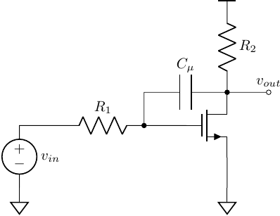 Example 01
the full transfer function is represented by
\[\begin{align} H(s) = \frac{H^{0} + \tau H^{1}s}{1 + \tau s} \end{align}\]$\square$
General Systems
For a \(n\)-th order system
\[\begin{equation*} H(s) = \frac{a_0 + a_1 s + a_2 s^2 + \dots}{1 + b_1 s + b_2 s^2 + \dots} \end{equation*}\] \[\begin{align*} b_1 &= -\sum_{i=1}^{N'}\frac{1}{p_i} = \sum_{i=1}^{N}\tau_{i}^{0}\\ b_2 &= \sum_{i}\sum_{j}^{1 \le i<j \le N} \tau_i^{0}\tau_{j}^{i}\\ b_3 &= \sum_{i}\sum_{j}\sum_{k} \tau_{i}^{0}\tau_{j}^{i}\tau_{k}^{ij} \\ &\dots \\ a_0 &= H^{0}\\ a_1 &= \sum_{i=1}^{N}H^{i}\tau_{i}^{0}\\ a_2 &= \sum_{i}\sum_{j}\tau_{i}^{0}\tau_{j}^{i}H^{ij}\\ a_3 &= \sum_{i}\sum_{j}\sum_{k}\tau_{i}^{0}\tau_{j}^{i}\tau_{k}^{ij}H^{ijk}\\ &\dots \end{align*}\]\(b_1\) Coefficient
If there are \(N\) energy storage elements (\(L\) or \(C\))
\[\begin{align} b_1 &= \sum_{i=1}^{N} \tau_{i}^{0} \end{align}\]- \(\tau_{i}^{0}\) is zero-valued time constant (ZVT) for energy storage element \(i\), when all the other elements are zero valued.
- zero \(C\) is equivalent to open circuit.
- zero \(L\) is equivalent to short circuit.
- the value of \(b_1\) may or may not reflect the bandwidth of \(H(s)\). I will use another post to explain bandwidth estimation techniques.
Example 02
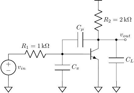 Example 02
Ignore \(r_o\) of the transistor and let
\[\begin{align} C_{\pi} &= 100 fF \quad \quad \quad r_{\pi} = 2.5 k\Omega \\ C_{\mu} &= 20 fF \quad \quad \quad \,\, g_{m} = 40 mS\\ C_{L} &= 200 fF \quad \quad \quad \beta = 100 \end{align}\]the time constants
\[\begin{align} \tau_{\pi}^{0} &= (R_1 \Vert r_{\pi}) C_{\pi} = (1k\Omega \Vert 2.5k\Omega) \cdot 100 fF = 70 ps\\ \tau_{\mu}^{0} &= (R_{left} + R_{right} + G_m R_{left} R_{right}) C_{\mu} = 1200 ps\\ \tau_{L}^{0} &= R_2 C_L = 400 ps \end{align}\]thus
\[b_1 = \tau_{\pi}^{0} + \tau_{\mu}^{0} + \tau_{L}^{0} = 1670 ps\]$\square$