From book_topics_in_the_theory_of_random_noise
Chapter 1: Random Functions and Their Statistical Characteristics
1. Random Variables
A random variable $\xi$ should have definition mean of any function \(\langle f(\xi)\rangle_{\xi}\)
\[\langle\xi\rangle_{\xi} = \lim_{n\to\infty} \dfrac{\xi_1 + \xi_2 + \dots + \xi_n}{n} = \lambda()\] \[\langle\xi^2\rangle_{\xi} = \lim_{n\to\infty} \dfrac{\xi_1^2 + \xi_2^2 + \dots + \xi_n^2}{n} = \lambda()\] \[\langle f(\xi)\rangle_{\xi} = \lim_{n\to\infty} \dfrac{f(\xi_1) + f(\xi_2) + \dots + f(\xi_n)}{n} = \lambda()\] \[\langle f(x,\xi)\rangle_{\xi} = \lim_{n\to\infty} \dfrac{f(x,\xi_1) + f(x,\xi_2) + \dots + f(x,\xi_n)}{n} = \lambda(x)\]- Derivitive: \(\dfrac{d}{dx}\langle f(x,\xi)\rangle_{\xi} = \langle \dfrac{\partial}{\partial x} f(x,\xi)\rangle_{\xi}\)
Integration: \(\int_{a}^{b}\langle f(x,\xi)\rangle_{\xi}dx = \langle\int_{a}^{b} f(x,\xi)dx\rangle_{\xi}\)
Assume we have a random variable \(\eta\), but it is actually fully determined by another random variable \(\xi\), \(\eta = g(\xi)\).
so, if \(\eta = g(\xi)\), then \(\langle f(\eta)\rangle_{\eta} = \langle f(g(\xi))_{\xi}\), or \(\langle f(g(\xi))\rangle_{g(\xi)} = \langle f(g(\xi))\rangle_{\xi}\)
if we define function
\[\theta(z) = \begin{cases} 1 & \text{ for } \quad z > 0,\\ 0 & \text{ for } \quad z \le 0 \end{cases}\]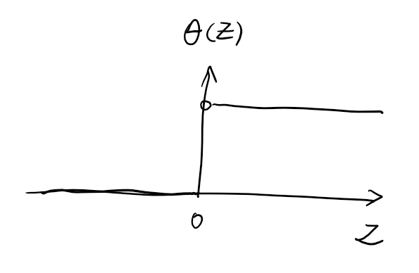
Then we have distribution function
\[P\{\xi < x\} = F_{\xi}(x) = \langle\theta(x-\xi)\rangle_\xi\]and the probability density function
\[\begin{align} w_\xi(x) &= \dfrac{d}{dx} F_\xi(x) = \dfrac{d}{dx}\langle\theta(x-\xi)\rangle_\xi = \langle\dfrac{\partial}{\partial x}\theta(x-\xi)\rangle_\xi = \langle\delta(x-\xi)\rangle_\xi \end{align}\]this can be used to calculate cany \(\langle f(\xi)\rangle\)
\[\begin{align} \langle f(\xi)\rangle_{\xi} &= \langle \int_{-\infty}^{\infty} f(x)\delta(x-\xi)dx \rangle_{\xi} = \int_{-\infty}^{\infty}\langle f(x)\delta(x-\xi)\rangle_{\xi} dx\\ &= \int_{-\infty}^{\infty} f(x)\langle\delta(x-\xi)\rangle_{\xi} dx = \int_{-\infty}^{\infty} f(x)w_{\xi}(x)dx \end{align}\]Next, we show how the probability density behaves under transformations of the original random variable \(\xi\). Let the new randon variable \(\eta\) be defined by
\[\eta = g(\xi)\]then
\[\begin{align} w_{\eta}(x) &= \langle\delta(x-\eta)\rangle_{\eta} = \langle\delta(x-g(\xi))\rangle_{\xi}\\ &= \int_{-\infty}^{\infty} \delta(x-g(\xi)) w_{\xi}(\xi)d\xi \end{align}\]If \(g(\xi)\) is monotone, it has a unique inverse function \(\xi = g^{-1}(\eta)\)
\[\begin{align} w_{\eta}(x) &= \int_{-\infty}^{\infty} \delta(x-g(g^{-1}(\eta)))w_{\xi}(g^{-1}(\eta))d(g^{-1}(\eta))\\ &= \int_{-\infty}^{\infty} \delta(x-\eta)w_{\xi}(g^{-1}(\eta)) \dfrac{dg^{-1}(\eta)}{d\eta}d\eta\\ &= w_{\xi}(g^{-1}(x))\dfrac{d g^{-1}(\eta)}{d\eta}\bigg|_{\eta=x}\\ &= w_{\xi}(\xi) \cdot (\dfrac{dg}{d\xi})^{-1}\bigg|_{\xi=g^{-1}(x)} \end{align}\]If there are multiple \(g(\xi_i) = x\)
\[w_{\eta}(x) = \sum_{i}\Bigg[ w_{\xi}(\xi_i)\cdot (\dfrac{dg}{d\xi})\bigg|_{\xi=\xi_i} \Bigg]\]Define characteristic function
\[\Theta_{\xi}(u) = \langle e^{iu\xi}\rangle_{\xi} = \int e^{iu\xi}w(\xi)d\xi\]this is similar to Fourier transform with only a sign different
\[w(\xi) = \dfrac{1}{2\pi}\int \Theta_{\xi}(u)e^{-iu\xi}du\]The moments \(m_n = \langle \xi^n\rangle_{\xi}\) can be calculated as
\[\begin{align} &\dfrac{1}{i^n}\dfrac{d^n \Theta_{\xi}(u)}{du^n}\bigg|_{u=0} = \dfrac{1}{i^n} \langle \dfrac{d^n}{du^n} e^{iu\xi} \rangle_{\xi}\bigg|_{u=0}\\ =& \dfrac{1}{i^n}\langle i^n \xi^n e^{iu\xi}\rangle_{\xi}\bigg|_{u=0} = \langle \xi^n\rangle_{\xi} \end{align}\]we can write \(\Theta_{\xi}(u)\) as a Maclaurin series:
\[\Theta_\xi(u) = 1 + \sum_{n=1}^{\infty} \dfrac{(iu)^n}{n!}m_n\]For a variaty of reasons, it is more convenient to characterize a random variable not by its moments, but by its cumulants (or semi-invariants) \(k_n\), defined by the relation
\[\Theta_{\xi}(u) = \exp \bigg\{ \sum_{n=0}^{\infty} \dfrac{(iu)^n}{n!}k_n \bigg\}\]using \(e^x = 1 + x + \dfrac{x^2}{2!} + \dfrac{x^3}{3!} + \dots\), comparing the two equations, we have, for example
\[\Theta_{\xi}(u) = 1 + \dfrac{iu}{1!}k_1 + \dfrac{(iu)^2}{2!}k_2 + \dfrac{(iu)^2}{2}k_1^2\]we can obtain the following formulas relating the moments and the cumulants:
\[\begin{align} k_1 &= m_1\\ k_2 &= m_2 - m_1^2\\ k_3 &= m_3 - 3m_1 m_2 + 2m_1^2\\ k_4 &= m_4 - 3m_2^2 - 4m_1 m_3 + 12 m_1^2 m_2 - 6m_1^4 \end{align}\]it shows
\[k_2 = \langle (\xi-\langle\xi\rangle)^2\rangle, \quad k_3 = \langle (\xi-\langle\xi\rangle)^3\rangle\]The quantity \(k_2 = \langle\xi^2\rangle - \langle\xi\rangle^2\) is called the variance (or dispersion) of \(\xi\), and is denoted by
\[\mathbf{D}\xi = \langle \xi^2\rangle - \langle\xi\rangle^2\]There are also defition for standard deviation
\[\sigma(\xi) = [\mathbf{D}\xi]^{1/2}\]2. Correlation Between Random Variables
Suppose we have \(r\) random variables \(\xi_1, \dots,\xi_r\), they are fully depends on a unknown random variable \(\zeta\)
\[\begin{align} \xi_1 &= g_1(\zeta)\\ \xi_2 &= g_2(\zeta)\\ & \dots \\ \xi_r &= g_r(\zeta) \end{align}\]then
\[\langle f(\xi_1,\dots,\xi_n)\rangle_{\zeta} = \lim_{n\to\infty} \dfrac{f(g_1(\zeta_1),\dots,g_r(\zeta_1))+\dots + f(g_1(\zeta_n)+\dots + g_r(\zeta_n))}{n}\]The random variables \(\xi_1,\dots,\xi_r\) are completely characterized by the (joint) \(r\)-dimensional probability density
\[w_{\xi_1,\dots,\xi_r}(x_1,\dots,x_r) = \langle \delta(\xi_1-x_1)\dots \delta(\xi_r - x_r) \rangle\]the mean value can be calculated as
\[\langle f(\xi_1,\dots,\xi_r) \rangle = \int \dots \int f(\xi_1,\dots,\xi_r) w(\xi_1,\dots,\xi_r) d\xi_1 \dots d\xi_r\]In the absence of knowledge of the actual realization (i.e., observed value) of \(\xi_2\), the random variable \(\xi_1\) has the probility density
\[w(\xi_1) = \int w(\xi_1,\xi_2)d \xi_2\]but
\[w(\xi_1 | \xi_2) = \dfrac{w(\xi_1,\xi_2)}{\int w(\xi_1,\xi_2)d\xi_1}\]If no information about \(\xi_1\) is gained, regardless of the observed value of \(\xi_2\), which means
\[\begin{align} w(\xi_1 | \xi_2) &= w(\xi_1)\\ w(\xi_1, \xi_2) &= w(\xi_1)w(\xi_2) \end{align}\]If \(\xi_1\) and \(\xi_2\) are completely correlated
\[w(\xi_1,\xi_2) = \delta[\xi_1 - f(\xi_2)]w(\xi_2)\]In general
\[\begin{align} w(\xi_1,\dots,\xi_k | \xi_{k+1},\dots,\xi_r) &= \dfrac{w(\xi_1,\dots,\xi_r)}{w(\xi_{k+1},\dots,\xi_r)}\\ w(\xi_1,\dots,\xi_k) &= \int \cdots \int w(\xi_1,\dots,\xi_r)d \xi_{k+1}\dots d\xi_{r} \end{align}\]The covariance (synonymously, cross correlation or double correlation) describe the degree of statistical dependence between random variables.
\[\mathbf{K}[\xi_1,\xi_2] = \langle \xi_1 \xi_2 \rangle - \langle \xi_1 \rangle \langle \xi_2 \rangle\]If \(\xi_1\) and \(\xi_2\) are independent, we have
\[\begin{align} \langle \xi_1 \xi_2 \rangle &=\langle \xi_1 \rangle\langle \xi_2 \rangle \mathbf{K}[\xi_1,\xi_2] &= 0 \end{align}\]By definition, the covariance of a random variable with itself is just its variance
\[\mathbf{K}[\xi,\xi] = \mathbf{D}\xi\]Sometimes, instead of \(\mathbf{K}[\xi_1,\xi_2]\)m it is convenient to consider the dimensionless quantity
\[R_2 \equiv R = \dfrac{\mathbf{K}[\xi_1,\xi_2]}{\sigma(\xi_1)\sigma(\xi_2)}\]The quantity reduces to unity when the random variables coincide, and is called the correlation coefficient of \(\xi_1\) and \(\xi_2\).
Besides double correlatoins, there are multiple correlations of higher orders. For example,
\[\langle \xi_1\xi_2\xi_3 \rangle - \langle \xi_1 \rangle\langle \xi_2 \rangle\langle \xi_3 \rangle\]But the triple correlation is defined as
\[\begin{align} \mathbf{K}[\xi_1,\xi_2,\xi_3] =\langle \xi_1 \xi_2 \xi_3 \rangle -\langle \xi_1 \rangle \mathbf{K}[\xi_2,\xi_3] -\langle \xi_2 \rangle \mathbf{K}[\xi_1,\xi_2] -\langle \xi_3 \rangle \mathbf{K}[\xi_1,\xi_2] -\langle \xi_1 \rangle\langle \xi_2 \rangle\langle \xi_3 \rangle \end{align}\]Chatacteristic function
\[\begin{align} \Theta(u_1,\dots,u_r) &=\langle \exp i(u_1 \xi_1 + \dots + u_r \xi_r) \rangle\\ \langle \xi_1,\dots,\xi_r \rangle &= \dfrac{1}{i^r} \dfrac{\partial^r \Theta(u_1,\dots,r_r)}{\partial u_1 \dots \partial u_r} \bigg|_{u_1 = \dots = u_r = 0}\\ \mathbf{K}[\xi_1,\dots,\xi_r] &= \dfrac{1}{i^r}\dfrac{\partial^r \ln \Theta(u_1,\dots,u_r)}{\partial u_1 \dots \partial u_r} \bigg|_{u_1=\dots=u_r=0} \end{align}\]3. Random Functions
Next, we consider a random function \(\xi(t)\) of a single real argument \(t\) (the time) which varies over the interval \([0, T]\), say.
If we take \(r\) fixed values \(t_1,\dots,t_r\) from the interval \([0,T]\), then the values \(\xi(t_1),\dots,\xi(t_r)\) constitute a family of random variables.
\[w_r(x_1,\dots,x_r;t_1,\dots,t_r) = \langle \delta[x_1-\xi(t_1)]\dots\delta[x_r-\xi(t_r)] \rangle\]The characteristic functions:
\[\begin{align} \Theta(u_1; t_1) &= \langle e^{i u_1 \xi(t_1)}\\ \Theta(u_1, u_2; t_1, t_2) &= \langle e^{i u_1 \xi(t_1)+iu_2\xi(t_2)} \rangle\\ &\dots \end{align}\]to the limit we get characteristic functional
\[\Theta[u(t)] = \bigg\langle \exp \bigg[i\int u(t)\xi(t) dt\bigg] \bigg\rangle\]The each characteristic function can be obtained by using
\[u(t) = \sum u_{\alpha} \delta(t-t_{\alpha})\]The term random process (or simply process) is used as a synonym for a random function of time.
In its general from, a random process cannot be described by a finite number of functions of a finite number of variables, and hence a random process is either characterized by an infinite sequence of functions or by a functional. It is preferable to consider a sequence of functions such that the functions of higher order do not repeat the information contained in the preceding functions, but instead carry only new information. Therefore, we now introduce another method of describing random processes, which has this and other advantages.
The mean values
\[\langle \xi(t_1)\dots\xi(t_r) \rangle = m_r(t_1,\dots,t_r)\]are called moment functions, and the infinite sequence of moment functions
\[m_1(t_1),\quad m_2(t_1,t_2),\quad m_3(t_1,t_2,t_3), \dots\]gives an exhaustive description of the random process \(\xi(t)\). It is even better to characterize the random process \(\xi(t)\) by the sequence of correlation functions
\[k_1(t_1),\quad k_2(t_1,t_2),\quad k_3(t_1,t_2,t_3), \quad\dots\]which are defined as the multiple correlations
\[k_r(t_1,\dots,t_r) \equiv \mathbf{K}[\xi(t_1),\dots,\xi(t_r)]\]regarded as functions of the time \(t_1,\dots,t_r\). The correlation functions, just like the moment functions, are symmetric functions of their arguments.
The vast majority of random processes encountered in radio physics have the property that when the time \(t_1,\dots,t_r\) are moved apart, the correlation between the corresponding values of the process falls off, i.e., the correlation functions goes to zero, which is very convenient.
If we know the moment functions or the correlation functions, we can find the other characteristics of a random process, in particular, its characteristic functions or probability densities.
Using formula \(\langle \xi_1,\dots,\xi_r \rangle = \dfrac{1}{i^r} \dfrac{\partial^r \Theta(u_1,\dots,r_r)}{\partial u_1 \dots \partial u_r} \bigg\vert_{u_1 = \dots = u_r = 0}\), we can write the characteristic function as a multidimentional Taylor’s series:
\[\Theta_r(u_1,\dots,u_r;t_1,\dots,t_r) = 1 + \sum_{s=1}^{\infty} \dfrac{s!}{i^s}\sum_{\alpha,\dots,\omega=1}^{r}m_s(t_{\alpha},\dots,t_{\omega})u_{\alpha}\dots u_{\omega}\]In just the same way
\[\Theta_r(u_1,\dots,u_r;t_1,\dots,t_r) = \exp \big\{\sum_{s=1}^{\infty} \dfrac{i^s}{s!} \sum_{\alpha,\dots,\omega=1}^{r} k_s(t_{\alpha,\dots,t_{\omega}})u_{\alpha}\dots u_{\omega}\big\}\]and
\[\Theta[u(t)] = \exp\big\{ \sum_{s=1}^{\infty} \dfrac{i^s}{s!} \int \cdots \int k_s(t_1,\dots,t_s) u(t_1) \dots u(t_s) d t_1 \dots d t_s \big\}\]Because of the special role played by moment functions and correlation functions, we give the following formulas relating them:
\[\begin{align} m_1(t_1) &= k_1(t_1)\\ m_2(t_1,t_2) &= k_2(t_1,t_2) + k_1(t_1)k_1(t_2)\\ m_3(t_1,t_2,t_3) &= k_3(t_1,t_2,t_3) + 3\{k_1(t_1)k_2(t_2,t_3)\}_s + k_1(t_1)k_1(t_2)k_1(t_3)\\ m_4(t_1,t_2,t_3,t_4) &= k_4(t_1,t_2,t_3,t_4) + 3\{k_2(t_1,t_2)k_2(t_3,t_4)\}_s + 4\{k_1(t_1)k_3(t_2,t_3,t_4)\}_s + 6\{k_1(t_1)k_1(t_2)k_2(t_3,t_4)\}_s + k_1(t_1)k_1(t_2)k_1(t_3)k_1(t_4) \end{align}\]Here, the symbol \(\{\dots\}_s\) denotes the operation of symmetrizing the expression in brackets with respect to all its arguments.
It seems like if \(k_1 = 0\), then the correlation functions are the same as the central moments. But it is not true. The difference begins with \(k_4\)
Chapter 2: Stationary Random Processes and Spectral Densities
A random process is said to be stationary (in the strict sense) if its statistical characteristics are invariant under time shifts, i.e., if they reamin the same when \(t\) is replaced by \(t+a\), where \(a\) is arbitrary. Then, the probability densities \(w_n(\xi_1,\dots,\xi_n;t_1,\dots,t_n)\) together with the moment and correlation functions \(m_n(t_1,\dots,t_n)\) and \(k_n(t_1,\dots,t_n)\) do not depend on the absolute position of the points \(t_1,\dots,t_n\) on the times axis, but only on their relative configuration.
\[k_n(t_1,\dots,t_n) = k_n(0,t_2-t_1,\dots,t_n-t_1) = k_n'(t_2-t_1,\dots,t_n-t_1)\]for which we introduce the special notation
\[k_2(t_1,t_2) = \langle \xi(t_1)\xi(t_2) \rangle - \langle \xi(t_1) \rangle \langle \xi(t_2) \rangle = k(t_2-t_1)\]where \(k(\tau) = k(-\tau)\). If the process has zero mean
\[k(\tau) = \langle \xi(0)\xi(\tau) \rangle\]We can also write \(k(\tau)\) in the form
\[k(\tau) = \sigma^2 R(\tau)\]where \(\sigma = \sigma[\xi(t)] = \sqrt{k(0)}\) is the standard deviation of \(\xi(t)\), and \(R(\tau) = k(\tau)/\sigma^2\) is the dimensionless, normalized correlation coefficient, with the property that \(R(0) = 1\).
Next, we introduce the important concept of the (power) spectral density \(S[\xi;\omega]\) of a stationary random process \(\xi(t)\):
\[S[\xi;\omega] = 2\int_{-\infty}^{\infty} e^{i\omega \tau} \langle \xi \xi_\tau \rangle d\tau = 4 \int_{0}^{\infty} \cos \omega \tau \langle \xi \xi_\tau \rangle d\tau\]Here, and subsequently, the subscript \(\tau\) on a function like \(\xi_\tau\), denotes a shift of the argument by a amount \(\tau\), i.e., \(\xi_\tau = \xi(t+\tau)\). For a process with zero mean value, \(S[\xi;\omega]\) is the Fourier transform of the correlation function:
\[S[\xi;\omega] = 2\int_{-\infty}^{\infty} e^{i\omega \tau} k(\tau) d\tau\]In the general case, where \(\langle \xi \rangle = m\) is not zero
\[\begin{align} S[\xi-m;\omega] &= 2\int_{-\infty}^{\infty} e^{i\omega\tau} k(\tau)d\tau\\ S[\xi;\omega] &= S[\xi-m;\omega] + 4\pi m^2 \delta(\omega) \end{align}\]The inverse formula gives
\[\sigma^2(\xi) = k(0) = \dfrac{1}{2\pi} \int_{0}^{\infty} S[\xi-m;\omega]d\omega\]